The Kalman Filter is a recursive algorithm invented in the 1960s to track a moving target from noisy measurements of its position and predict its future position. The Kalman filter is an optimal estimation algorithm and is a type of state observer, but it is designed for stochastic systems.
The Kalman Filter works in two stages:
- Predict current state based on last state, taking noise into account
- Update: takes measured values, and updates the state estimate
The Kalman Filter is adaptive and may be a more accurate smoothing/prediction algorithm than the simple moving average. The calculation accounts for estimation errors and adjusts its predictions from the information it calculated in the previous stage.
The study has only one parameter besides the choice of market data to use, i.e., close and that parameter is NoiseCovRatio.
The parameter NoiseCovRatio is a ratio of measurement noise to process noise variance. Large values of NoiseCovRatio make trend smoother, but slow down reaction to the change in trend. Small values of NoiseCovRatio make noise smoothing worse but keeps good reaction to the change in trend.
This first image displays the E-mini-Nasdaq 100 contract (symbol: ENQ,ADC) with the Kalman Filter applied using a Noise Cover Ratio (NoiseCovRatio parameter) set to 10.
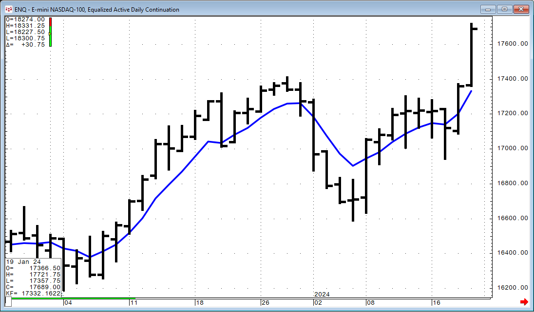
Theoretically, the Kalman Filter consists of measurement and transition components. The measurement component relates an unobservable price trend to the observable price variable. Referred to as the measurement noise, it is manifested as a deviation of predicted to actual price. The transition component specifies the price trend to either increase or decrease. Referred to as the process noise variance, it is manifested as the price smoothing component. Observing the image above, the Kalman Filter does appear to be sensitive to both the trend and a change in the direction of the trend, similar to an Exponential Smoothed Moving average (EMA). This next image displays both the Kalman Filter (blue line) and the 10-period EMA (red line).

We can see that the EMA does lag the market more than the Kalman Filter. The next image includes a 10-period Simple Moving Average (green line).
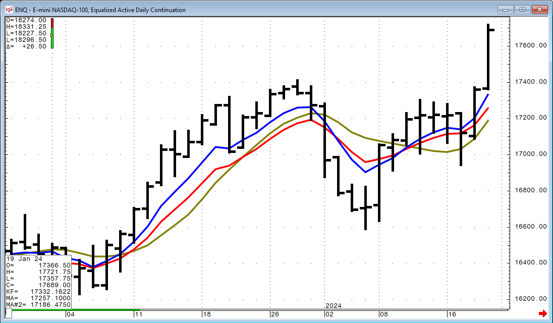
The 10-period Simple Moving Average shows more lag than both the Kalman Filter and the EMA.
A possible use of the Kalman Filter is to substitute the Kalman Filter value for the closing price in a trading system. For example, if the closing price is above the 100-period simple Moving Average, the market trend is up. And, if the value of the Kalman Filter at the close drops below the close of the 5-period Simple Moving Average then the market is in a pullback and go long. Stay long until the condition is no longer true.
This next image shows some recent trading activity.

A CQG PAC with this system is available at the bottom of the post for further development.
Also, at the bottom of the post is an Excel sample spreadsheet to pull in the Kalman Filter data using the following formula:
= RTD("cqg.rtd",,"StudyData", "KF("&$L$2&",NoiseCovRatio:=10,InputChoice:=Close)", "BAR", "", "Close", $L$4, -$A2, $L$6,$L$10,,$L$8,$L$12)
For more information detailing the aspects of the Kalman Filter using non-market examples MathWorks has a collection of videos.
Requires CQG Integrated Client and Excel 2016 or more recent.