This article walks through the details of using three Microsoft Excel® functions: RANK, COUNTIF, and VLOOUP. These functions are used to build an Excel dashboard that automatically ranks a collection of markets based on percent net change and then displays the market symbols ranked from first to last in a column. A downloadable Excel sample is provided.
The advantage of dynamically ranking a group of markets by percent net change is it allows the trader to simply see what is strong and what is weak without having to compare values from cell to cell.
Excel offers the Rank function whereby you can see where the value in one cell is in the ranked order of a collection of cells in a column. Below, column A are example symbols for five markets, column B has the five markets net percent change in cells B1 through B5. The Rank function in cell C1 would be:
=RANK(B1,$B$1:$B$5,0)
You copy and paste this formula in cell C1 down to cell C5. The Rank function displayed above is checking the rank order for cell B1 in the reference range of $B$1 to $B$5. Using dollar signs locks the range to always be B1 to B5 when you copy and paste down. The “0” indicates the results to be in ascending order, i.e., first, second, third, and so on. Use “1” if you want the results to be in descending order. Column C displays the rank:
| A | B | C | |
| 1 | A | 0.12% | 5 |
| 2 | B | 0.55% | 1 |
| 3 | C | 0.12% | 4 |
| 4 | D | 0.31% | 3 |
| 5 | E | 0.44% | 2 |
However, the Excel Rank function assigns ties with the same value, as shown below with updated net percent changes for symbols C and D. Now, both are displaying a rank of 3 in column C:
| A | B | C | |
| 1 | A | 0.12% | 5 |
| 2 | B | 0.55% | 1 |
| 3 | C | 0.31% | 3 |
| 4 | D | 0.31% | 3 |
| 5 | E | 0.44% | 2 |
For many uses, a tie assigned to the same value is not an issue. Here we will be using VLOOKUP, and if there is a tie, then it is a problem as VLOOKUP will generate an error. However, by using an additional function, COUNTIF, with the RANK function then ties will automatically be assigned the next value in the order rank. Below is the COUNTIF function:
COUNTIF($B$1:B1,B1)
Here, COUNTIF is looking in range B1 to B1 and how many times the value from cell B1 occurs. Obviously, the value in B1 can only appear once in a range of B1 to B1. Notice, the dollar sign is only used in the first part of the range. When this formula is copied and pasted down, then the start of the range is always B1 but the bottom of the range will be dependent on how far down the formulas is copied and pasted. In our example, it would be using a range down to cell B5:
COUNTIF($B$1:B5,B5)
Here is the modified version of the ranking function which includes COUNTIF and is entered into cell C1 and copied and pasted down to cell C5 (Courtesy of Chip Pearson's site):
=RANK(B1,$B$1:$B$5,0)+COUNTIF($B$1:B1,B1)-1
COUNTIF checks for how many times a value occurs in a range. In our example, 0.31% occurred twice. So, COUNTIF would return two and one is subtracted from two and added to the RANK function. This additional step removes ties:
| A | B | C | |
| 1 | A | 0.12% | 5 |
| 2 | B | 0.55% | 1 |
| 3 | C | 0.31% | 3 |
| 4 | D | 0.31% | 4 |
| 5 | E | 0.44% | 2 |
We can see that the first time 0.31% occurs its rank is three and the second time it occurs the rank is four.
Let’s add the symbols next to the ranking in column D and integers 1 to 5 in column E and now use VLOOKUP:
| A | B | C | D | E | |
| 1 | A | 0.12% | 5 | A | 1 |
| 2 | B | 0.55% | 1 | B | 2 |
| 3 | C | 0.31% | 3 | C | 3 |
| 4 | D | 0.31% | 4 | D | 4 |
| 5 | E | 0.44% | 2 | E | 5 |
In Column F we use VLOOKUP. VLOOKUP finds the value in a range (column) and then can return information that is next to the value in the range. In Cell F1 we have:
=VLOOKUP(E1,$C$1:$D$5,2,FALSE)
Excel looks for the value in cell E1 within the range C1 through D5. Each column has an index value. Column C is index value 1 and column D is index value 2. and we want the information that is the second column to the right of C1, which will be “B”. FALSE indicates it has to be an exact match. Copying and pasting down the VLOOKUP formulas to cell F5 produces a ranked list of the symbols:
| A | B | C | D | E | F | |
| 1 | A | 0.12% | 5 | A | 1 | B |
| 2 | B | 0.55% | 1 | B | 2 | E |
| 3 | C | 0.31% | 3 | C | 3 | C |
| 4 | D | 0.31% | 4 | D | 4 | D |
| 5 | E | 0.44% | 2 | E | 5 | A |
Column F are the ranked symbols by percent net change. Now, we can use the ranked symbols for more market information.
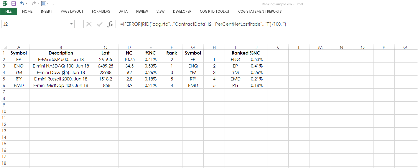
The downloadable sample spreadsheet uses RTD calls for five CME products and the above Excel Rank, COUNTIF and VLOOKUP formulas. The source for this article is http://www.cpearson.com/Excel/Topic.aspx.