This post details how to extract data from a large array, such as a correlation matrix, to make your workflow more efficient.
First, as the LAMBDA function is used, a brief overview is provided.
Excel 365 offers the LAMBDA function, which was detailed here.
The LAMBDA function features are threefold:
- Assign parameters.
- Pass the parameters to a function.
- Assign the function a "friendly name."
Two functions are available for use with the LAMBDA function: BYCOL and by BYROW. This post details examples of using the three functions and a downloadable Excel spreadsheet sample is available at the bottom of this post. The subject of the application of the three functions is an Excel correlation matrix.
Correlation analysis by technical traders is a popular analytical technique for identifying opportunities. Excel RTD formulas can pull the data correlation values directly from CQG IC and QTrader instead of having Excel do the analysis.
The RTD formula requires two symbols, a lookback period parameter, choice of markets' data (such as the "close,"), and the time interval (i.e. 5, 10, D):
=RTD("cqg.rtd",,"StudyData", "Correlation(Symbol 1,Symbol 2,Period:=10 ,InputChoice1:=Close,InputChoice2:=Close)", "Bar", "", "Close", Time Interval, "0", "all","", "","True","T")/100
In cell C4 in the sample spreadsheet the two symbols are in cells C3 and B4, the period is from cell C2 and the interval is from cell E2. This formula is copied and pasted to cells B4 to S21:
=RTD("cqg.rtd",,"StudyData", "Correlation("&C$3&","&$B4&",Period:="&$C$2&",InputChoice1:=Close,InputChoice2:=Close)", "Bar", "", "Close",$E$2, "0", "all","", "","True","T")/100

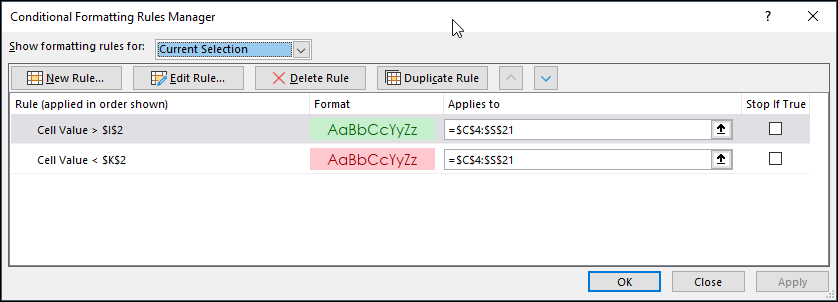
Generally, correlation is interesting when values are very positive, such as greater than 0.90 or very negatives, such as less than -0.90. The sample spreadsheet uses color conditioning:
- Correlations greater than 0.90 are highlighted with green backgrounds.
- Correlations less than -0.90 are highlighted with red backgrounds.
To add the color coding the steps are select the area for the color coded conditioning go to Home/Conditional Formatting/Hight Cell Rules/Greater Than cell $I$2 is selected as that has the threshold and select the colors.

Repeat that for less than, the threshold cell reference is $K$2. You can manage the feature by selecting the same area and going to Home/Conditional Formatting/Manage Rules.
However, the user has to peer at the spreadsheet and visually trace upwards to find one symbol and visually trace to the left to identify the second symbol. A better solution is to have Excel extract the group of symbols from the greater than 0.90 group and the less than -0.90 group. The LAMBDA function plus BYCOL and BYROW functions will do this.
This will be a two step process. First, in the sample spreadsheet cell U23 is referencing cell B4 for the symbol and copied down to cell U40.
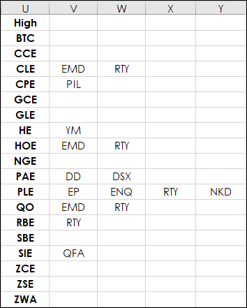
Next, using the BYCOL and the LAMBDA functions Excel will determine the columns with greater than 0.90 correlations. The LAMBDA function is counting the number of times the cells C4:S4 is greater than 0.90 and the Filter function returns the symbol in cells $C$3:$S$3. This formula is entered into cell V23 and copied down to V40.
=FILTER($C$3:$S$3,BYCOL(C4:S4,LAMBDA(High,COUNTIF(High,">"&$I$2)))>0,"")
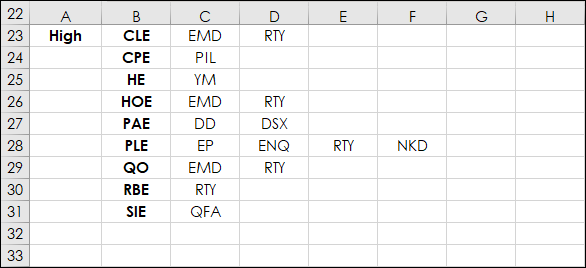
Next, based on the first step, then using the BYROW and the LAMBDA functions Excel will return the symbols with the rows with greater than 0.90 correlations. This formula is entered into cell B23 and is not copied down. The symbols will "Spill" down. Important note: Leave cells blank from cell B24 to Cell B40 otherwise you will see the "Spill error".
=FILTER(B4:B21,BYROW(C4:S21,LAMBDA(High,COUNTIF(High,">"&$I$2)))>0)
Next, now that Excel provides the symbols with correlations higher than 0.90 by the symbol columns, as shown in the image above, and Excel lists the symbols by rows, what would be useful is to have only both the symbols by rows and the symbols by columns. To that end, the IFS function and the INDIRECT function are key, i.e.:
=IFS(B23=$B$4,INDIRECT("V23:AL23"),B23=$B$5,INDIRECT("V24:AL24")...Above the IFS function is an IF THEN function and will stop at the first IF that is True. The INDIRECT function pulls data from a row using Text to state the parameters of the row.
Pulling in data by the roll will deliver "0" if there is no symbol, so the TEXT function is used to only display text. The formula below is in cell C23 and copied down to cell C40. The IFERROR function is used to display a blank cell if there is not a symbol in column B.
=IFERROR(TEXT(IFS(B23=$B$4,INDIRECT("V23:AL23"),B23=$B$5,INDIRECT("V24:AL24"),B23=$B$6,INDIRECT("V25:AL25"),B23=$B$7,INDIRECT("V26:AL26"),B23=$B$8,INDIRECT("V27:AL27"),B23=$B$9,INDIRECT("V28:AL28"),B23=$B$10,INDIRECT("V29:AL29"),B23=$B$11,INDIRECT("V30:AL30"),B23=$B$12,INDIRECT("V31:AL31"),B23=$B$13,INDIRECT("V32:AL32"),B23=$B$14,INDIRECT("V33:AL33"),B23=$B$15,INDIRECT("V34:AL34"),B23=$B$16,INDIRECT("V35:AL35"),B23=$B$17,INDIRECT("V36:AL36"),B23=$B$18,INDIRECT("V37:AL37"),B23=$B$19,INDIRECT("V38:AL38"),B23=$B$20,INDIRECT("V39:AL39"),B23=$B$21,INDIRECT("V40:AL40")),"#"),"")This is the display reduced to just symbols with correlations greater than 0.90.
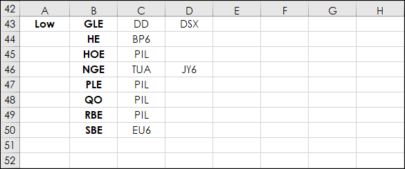
For the less than -0.90 group the symbols are referenced in Cell U43 to Cell U60 from cell B4 down to B21. Here the LAMBDA function is using Low referenced in cell $K$2.
=FILTER($C$3:$S$3,BYCOL(C4:S4,LAMBDA(Low,COUNTIF(Low,"<"&$K$2)))>0,"")
Resulting in this display.

Then in cell B43 this function is entered (do not copy down).
=FILTER(B4:B21,BYROW(C4:S21,LAMBDA(Low,COUNTIF(Low,"<"&$K$2)))>0,"")
And this function is used in cells C43 to C60.
=IFERROR(TEXT(IFS(B43=$B$4,INDIRECT("V43:AL43"),B43=$B$5,INDIRECT("V44:AL44"),B43=$B$6,INDIRECT("V45:AL45"),B43=$B$7,INDIRECT("V46:AL46"),B43=$B$8,INDIRECT("V47:AL47"),B43=$B$9,INDIRECT("V48:AL48"),B43=$B$10,INDIRECT("V49:AL49"),B43=$B$11,INDIRECT("V50:AL50"),B43=$B$12,INDIRECT("V51:AL51"),B43=$B$13,INDIRECT("V52:AL52"),B43=$B$14,INDIRECT("V53:AL53"),B43=$B$15,INDIRECT("V54:AL54"),B43=$B$16,INDIRECT("V55:AL55"),B43=$B$17,INDIRECT("V56:AL56"),B43=$B$18,INDIRECT("V57:AL57"),B43=$B$19,INDIRECT("V58:AL58"),B43=$B$20,INDIRECT("V59:AL59"),B43=$B$21,INDIRECT("V60:AL60")),"#"),"")This is the current result.
Using the combination of BYCOL, BYROW and the LAMBDA functions can extract data from a large array and reduce it to a more usable display. Again, for those functions that "SPILL" you need to leave empty cells so the functions can properly populate with data.
You can use your own symbols in cells C3 to S3 and Cells B4 to B 21.
Requirements: CQG Integrated Client or QTrader, and Excel 365 (locally installed, not in the Cloud) or more recent.