Microsoft® Office 365 includes the latest version of Excel which comes with some new functions not available in Excel 2016 or Excel 2019. This post details the XLOOKUP function and its features. Note: Excel must be installed on your computer (not in the Cloud) for Excel to connect with CQG IC or QTrader and deliver data to Excel via the RTD formulas.
The XLOOKUP function searches a range or an array, and then returns the data corresponding to the first match it finds. If no match exists, then XLOOKUP can return the closest (approximate) match or a user defined input if an approximate match is not available.
XLOOKUP is superior to VLOOKUP and HLOOKUP. For example, VLOOKUP required the lookup value to be to the left of the lookup array and the return array. XLOOKUP does not have that requirement. HLOOKUP required the row number as a parameter, XLOOKUP does not. Here is the function and parameters:
=XLOOKUP(lookup_value, lookup_array, return_array, [if_not_found], [match_mode], [search_mode])
This table describes the parameters including required or optional.
| Parameter | Description |
|---|---|
| lookup_value | The value to search for in the lookup_array. |
| Required* | *If omitted, XLOOKUP returns blank cells it finds in lookup_array. |
| lookup_array | The array or range to search. |
| Required | |
| return_array | The array or range reviewed to return the data. |
| Required | |
| [if_not_found] | When a valid match is not found, return the [if_not_found] text the user supplies. |
| Optional | If a valid match is not found, and [if_not_found] is missing, the error #N/A is returned. |
| [match_mode] | Specify the match type by using one of the following numerical inputs: |
| Optional | 0: Exact match. If none is found, then return the error #N/A. This is the default. -1: Exact match. If none found, return the next smaller item. 1: Exact match. If none found, return the next larger item. 2: A wildcard match where *, ?, and ~ have a special meaning. |
| [search_mode] | Specify the search mode to use by using one of the following numerical inputs: |
| Optional | 1: Perform a search starting at the first item. This is the default. -1: Perform a reverse search starting at the last item. 2: Perform a binary search that relies on lookup_array being sorted in ascending order. If not sorted, invalid results will be returned. -2: Perform a binary search that relies on lookup_array being sorted in descending order. If not sorted, invalid results will be returned. |
Two Excel samples are provided at the bottom of the post. The first is an application of the XLOOKUP function in a basic form. The second uses the XLOOKUP function in conjunction with a drop-down selection choice and the Excel Indirect function.
The XLOOKUP function is replacing the VLOOKUP function. The VLOOKUP function requires a column parameter in the table for the return array and declaring whether the match is a perfect match or not. Using XLOOKUP function requires an array or range for the return array (not a column number) and perfect match is the default parameter.
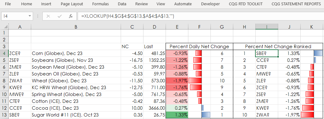
The Simple Sample is analyzing a small portfolio using net percentage change, ranking the contracts by net percent change, and then sorting the contracts using XLOOKUP from highest to lowest.
The ranking of the net percentage change (cells E4:E13) is performed in cells G4:G13. The Excel Rank function will assign ties with the same rank and that leads to an error returned when using XLOOKUP to sort the ranked values. Including COUNTIF will replace a tie with the next value.
=IFERROR(RANK(E4,$E$4:$E$13,0)+COUNTIF($E$4:E4,E4)-1,"")
The XLOOKUP function is using numbers 1 through 10 in cells H4:H13, the ranking score from cells G4:G13, and is first pulling the symbols from cells A4:A13:
=XLOOKUP(H4,$G$4:$G$13,$A$4:$A$13,"")
Again, using numbers 1 through 10 in cells H4:H13, the ranking score from cells G4:G13, and the percentage net change from cell E4:E14:
=XLOOKUP(H4,$G$4:$G$13,$E$4:E$13,"")
Cells K4:K13 are simply the values from cells J4:J13 and the data histogram bars are applied from conditional formatting.
The Sample XLOOKUP is like the simple sample but has multiple groups of markets, and displays Daily, Weekly, Monthly, and Percent Annual Net change.
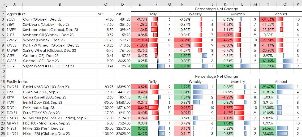
In addition, to the right (displayed below) is a section where the percent net change is sorted. There is a drop-down menu to choose Daily, Weekly, Monthly or Annual percent net change.
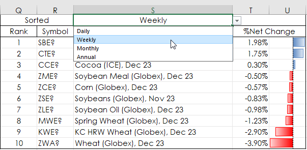
Here, the XLOOKUP function, depending on the choice from the drop-down menu, is using the INDIRECT function for the Look-up range. The Look-up range is in cell $AB$2. If you modify the number of rows in the table by either adding or deleting a symbol, then the cells in column AB will need to be modified.
=IF($S$1="Daily",XLOOKUP(Q3,INDIRECT($AB$2),$B$3:$B$12,""),IF($S$1="Weekly"…
Also, following “$B$3:$B$12” above is ,””. That parameter is used when there is an error and is displaying a blank cell.
XLOOKUP is an added Excel function in Excel 365 and is worthwhile using.
Requirements: CQG Integrated Client or QTrader, and Excel 365 (locally installed, not in the Cloud) or more recent.