This article walks you through using Microsoft® Excel’s LINEST function to determine the three coefficients and y-intercept of a 3rd order polynomial function over the past 20 bars of closing price data. In addition to the downloadable sample Excel spreadsheet, a CQG PAC is provided that uses the XLTS study to pull the results into CQG to display on a chart.
The Third Order Polynomial Trend line has this mathematical formula:
y = (c3 * x^3) + (c2 * x^2) + (c1 * x^1) + b
Where Excel calculates the three coefficients, x is the x-axis values and b is the y intercept.
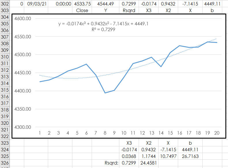
Here is an example of applying this trend line to a daily close line chart of data (symbol: EP) in Excel. Ultimately, the Y value (end point) will be displayed in CQG on the chart.
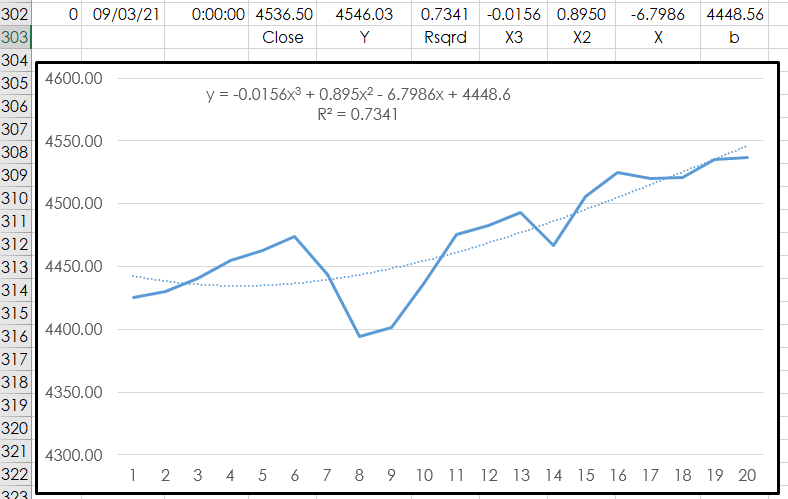
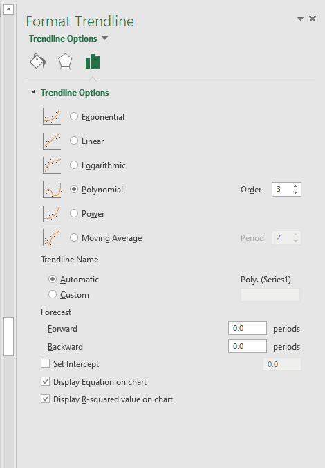
To add this Trend line to an Excel chart right-click on the line and select “Add Trend line’ and make the selection, here a 3rd order polynomial trendline is the choice. In addition, “Display Equation on chart” and “R-squared value on chart” are checked. You can see in the above image that the bottom row of values displayed in row 302 match the values on the chart. In addition, note the X-axis data are integers from 1-20, not dates or time.
The Excel formula for a 3rd order polynomial:
=LINEST(D2:D21,$K$2:$K$21^{1,2,3},,TRUE)Column D are the closing prices. Cells “$K$2:$K$21” are a fixed reference and are integers 1 through 20 for the X-axis. The “^{1,2,3},,” are the parameters for a third order polynomial. The “TRUE” is an instruction to return additional regression statistics such as R-squared.
The Excel LINEST formula is entered as an array, which is a collection of cells that populate with the various regression values and cannot be edited. Looking at the image of the chart the values displayed below the chart are the returned values when the function is entered as an array. The coefficients are in row 1 column 1, row 1 column 2, and row 1 column 3. The b values i in row 1 column 4. The R-squared value is in row 3 column 1.
A valuable feature in Excel is the “Index” function. The Index function allows you to request a value from an array by the row and column reference.
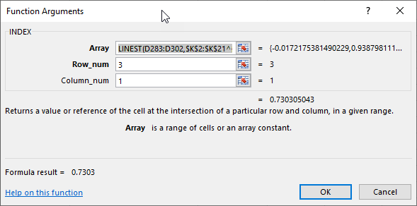
For example, in row 302 in the screen capture of Excel and the chart the first, second and third coefficients are:
Cell G 302: =INDEX(LINEST(D283:D302,$K$2:$K$21^{1,2,3},,TRUE),1)
Cell H 302: =INDEX(LINEST(D283:D302,$K$2:$K$21^{1,2,3},,TRUE),1,2)
Cell I 302: =INDEX(INDEX(LINEST(D283:D302,$K$2:$K$21^{1,2,3},,TRUE),1),1,3)The b value is:
Cell J 302: =INDEX(INDEX(LINEST(D283:D302,$K$2:$K$21^{1,2,3},,TRUE),1),1,4)And, the R-squared value is:
Cell F 302: =INDEX(LINEST(D283:D302,$K$2:$K$21^{1,2,3},,TRUE),3,1)The Y value is calculated in column E:
Cell E 302: =G302*(20^3)+H302*(20^2)+I302*20+J302
The Top of the Spreadsheet
The above formulas are detailing the bottom row of the spreadsheet. The top of the spreadsheet allows you to enter in a symbol (all capital letters), time frame, equalize closes (True or False), All sessions or just the primary session, use a custom session, and the price format is either decimal (T) or no price formatting (D).
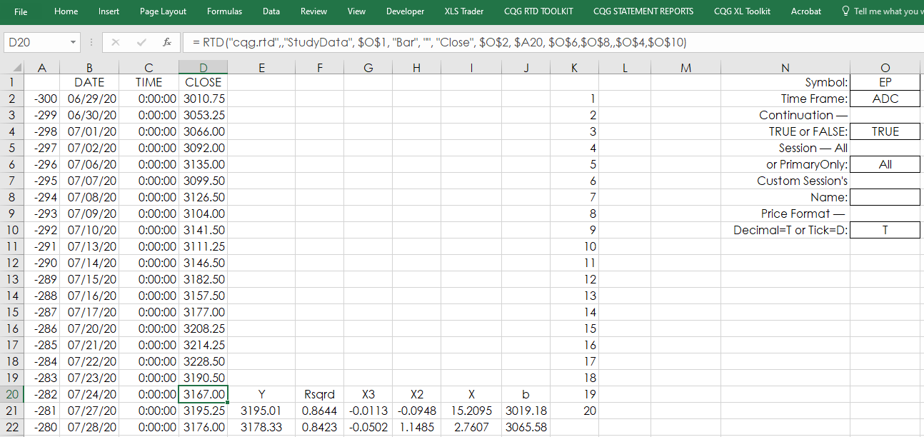
Columns B, C and D use standard RTD formulas to pull in the dates, times and closing prices. Columns E through Z display the polynomial data and the R-squared values. Column K is the fixed references for the 20-bar lookback. The same formulas used for row 302 are used for row 21 except the closing prices start at D2:D21.
The Date/Time (column B) and Y values (Column E) are pulled into the Chart tab, as well as column F’s R-Squared values access by the XLTS study in CQG.
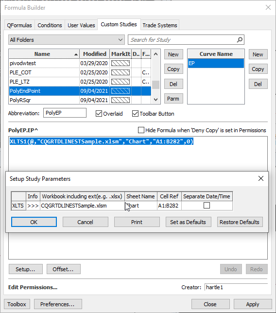
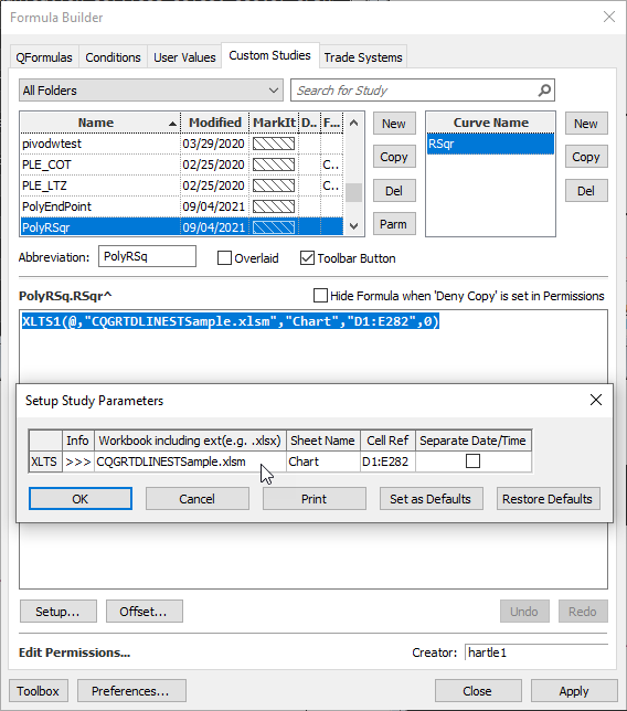
The XLTS Study
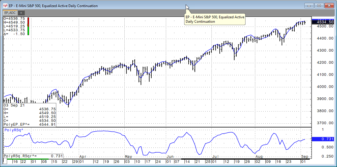
The XLST study pulls in times series data from Excel to be displayed on a CQG chart. The study requires the full name of the spreadsheet including the extension, the name of the Sheet and the columns (one is date/time and the second is data). The Y value of the polynomial is plotted, which is the end point of the polynomial, and is displayed as an overlay chart.
The second XLST Study is the R-squared value and is displayed in its own pane.
Below is the chart with the two studies. When the PAC is installed, it will create a unique page.
The symbol and time frame for the chart and the Excel spreadsheet must match. For equities, use the number of minutes in the session, such as “405” or “390”, not “D”.
Requires CQG Integrated or QTrader. Strongly recommended: Microsoft Office Professional Excel 2016, 2019, 32 or 64-bits installed on your computer, not in the Cloud.