This post walks you through using Microsoft® Excel’s Indirect function and other Excel features to make usable Quote Dashboards. The provided sample Excel spreadsheet is unlocked.
Consider that you may have multiple tabs for different markets and you want a way to pull in data from one of the tabs by selecting the tab name from a dropdown list. The dropdown list combined with the Indirect function is one solution.
The Indirect Function can return a value based on a text string. For example, If in cell A1 on Sheet1 this formula was entered:
=INDIRECT("Sheet2"&"!A1")
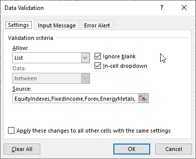
This formula returns the value from Sheet2, cell A1. The Excel sample supplied has a dropdown list in cell B3 and cell B20 on the main display tab.
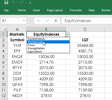
The dropdown list source is using the names of the tabs in the sample Excel spreadsheet. The source could also be a range of cells with the name of the tabs.
The two dropdown lists are used by the Indirect function. For example, in cell A3 the function is:
=INDIRECT($B$1&"!A2")
In cell B1 is EquityIndexes, which is the name of the tab and the function is pull in the value in A2, which is the symbol YM2. Selecting a different named tab in the dropdown list will update the MainDisplay tab with that market data. The MainDisplay tab updates all values based on the tab name listed in cell B1 or B20 selected by the user.
Formatting Prices
The following applies to the tabs other than the MainDisplay tab.
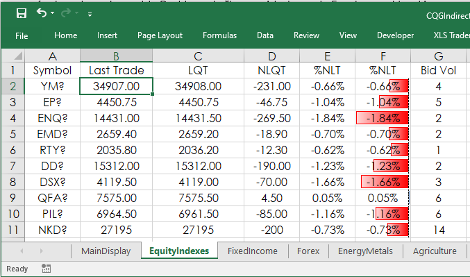
Excel does not know that the symbol for the E-mini S&P 500 contract uses two decimal places for the price or that the symbol for the Euro FX contract uses 5 decimal places for the price. The price formatting can be done manually in Excel. However, using Excel’s IF function combined with Excel’s Text function offers automatic price formatting.
First, the RTD contract label has four parameters for price formatting, this spreadsheet uses two: B and T.
= RTD("cqg.rtd", ,"ContractData", “TYA”, "TradeorTodaySettlement",,"B") = RTD("cqg.rtd", ,"ContractData", “TYA”, "TradeorTodaySettlement",,"T")
B is for bond data (fractions) and T is for decimals.
Using B for the 10-year T-Note last trade returns 125-23'+ and using T returns 125.734375.
Our first goal is to determine if the symbol is a T-Note (or T-Bond) or everything else, which will use decimals. The Notes/Bonds symbols have a tick size that is based on 32nds. On the non-MainDisplay tabs in column O this RTD formula is used:
=RTD("cqg.rtd",,"ContractData",A2,"TickSize",, "T")
The above RTD formulas pulls the tick size for the symbol in cell A2. This table lists the tick sizes for the Two Year T-Note, Five Year T-Note, Ten Year T-Note and the Thirty Year T-Bond:
TUA?
0.00390625
FVA?
0.0078125
TYA?
0.015625
USA?
0.03125
To determine if a symbol is a fixed income instrument for price formatting we use this IF Or function in column P:
=IF(OR(O2=0.00390625,O2=0.0078125,O2=0.015625,O2=0.03125),"B","T")
If the symbol has one of these values for a tick size it is a fixed income instrument and uses B for all of the price formatting, otherwise T is used for the price formatting.
Next, if you use Excel formatting set to “General” then, for example, the E-Mini S&P could display these three different prices: 4470, 4470.25, and 4470.5, which is a little annoying because the prices are jumping sideways back and forth. One solution is the cell could be manually set to always display two decimals.
The solution used in this sample spreadsheet is to count the number of digits to the right of the decimal for the tick size and convert the value to Text using Excel’s Text function with a decimal format applied based on the number of digits to the right of the decimal. Column Q looks at the length of the tick size and subtracts 2 for the count (not using the 0 and the decimal):
=LEN(O2)-2)
As is always the situations with computers and markets there are “edge cases.” To deal with edge cases the actual formula used in column Q is:
=IF(P2="B","",IF(O2=1,2,IF(O2=0.1,2,IF(O2=0.5,2,IF(O2=5,0,LEN(O2)-2)))))
So, if the symbol is a fixed income instrument then a blank space is returned, If the tick size is 1 or 0.1 or 0.5 then a 2 for the decimal place is returned and if the tick size is 5 a 0 is returned. Otherwise, LEN(O2)-2) is used.
The values returned in column Q are used for the Text Function and the price formatting. The Text function lets you set how many decimal places to use, such as =TEXT(100.285,"0.##") = 100.29. Just two decimal places are used and are rounded up. We do not want to use rounding.
Column R has this formula:
=IF(P2="B","",IF(Q2=0,"#",IF(Q2=1,"#.0",IF(Q2=2,"#.00",IF(Q2=3,"#.000",IF(Q2=4,"#.0000",IF(Q2=5,"#.00000",IF(Q2=6,"#.000000",IF(Q2=7,"#.0000000",IF(Q2=8,"#.0000000"))))))))))
All of the market prices on these tabs use this column for setting the price formatting. For example, in cell B2 for Trade Today or Settlement:
=IFERROR(IF(P2="B",RTD("cqg.rtd", ,"ContractData", A2, "TradeorTodaySettlement",,"B"),TEXT(RTD("cqg.rtd", ,"ContractData", A2, "TradeorTodaySettlement",,"T"),R2)),"")
The IFERROR function returns a blank space to keep the dashboard looking clean and is used throughout the spreadsheet.
Summary
This article walked you through using Excel’s INDIRECT function to allow market data to be displayed based on a dropdown list, as well as tips for automatically formatting prices for fixed income markets or for markets that use decimal formatting.
Requires CQG IC or QTrader and Excel 2013 or higher installed on your computer, not in the Cloud.