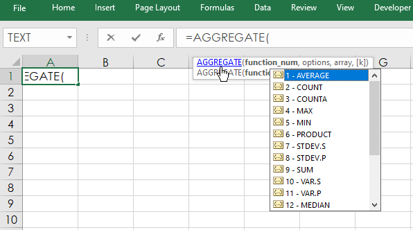
The Excel AGGREGATE function returns an aggregate calculation such as AVERAGE, COUNT, COUNTA, MAX, MIN, PRODUCT, etc., applied to a list of data while optionally ignoring hidden rows and errors. Nineteen operations are available. The choice is specified by the function number in the first argument. This image displays a partial list from the drop-down menu for AGGREGATE.
This table below is the full list of options. The first column is the function number used in the formula, the second column is the function and the third column lists if there is an additional parameter required.
| Function Number 1 | Function | Function Number 1 |
|---|---|---|
| 1 | AVERAGE | |
| 2 | COUNT | |
| 3 | COUNTA | |
| 4 | MAX | |
| 5 | MIN | |
| 6 | PRODUCT | |
| 7 | STDEV.S | |
| 8 | STDEV.P | |
| 9 | SUM | |
| 10 | VAR.S | |
| 11 | VAR.P | |
| 12 | MEDIAN | |
| 13 | MODE.SNGL | |
| 14 | LARGE | k |
| 15 | SMALL | k |
| 16 | PERCENTILE.INC | k |
| 17 | QUARTILE.INC | quart |
| 18 | PERCENTILE.EXC | k |
| 19 | QUARTILE.EXC | quart |
For example, function 14 is LARGE and there is an additional parameter “k”.
Here, is the Function Arguments for LARGE and setting K = 5 then the fifth largest number in the array is returned. If K is not declared in the AGGREGATE function an error is returned.
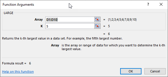
These two functions return the same value.
=LARGE(D1:D10,5)
=AGGREGATE(14,6,D1:D10,5)
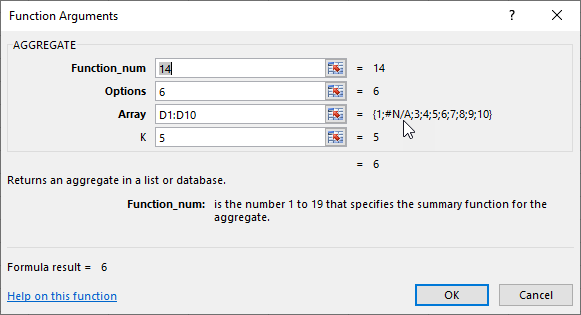
Notice the number 6 after the Function Number. This parameter is the real value of using the AGGREGATE function as it sets the behavior in case of an issue such as there is an error in the data array. This table lists the choices available.
| Option | Behavior |
|---|---|
| 0 or omitted | Ignore nested SUBTOTAL and AGGREGATE functions |
| 1 | Ignore hidden rows, nested SUBTOTAL and AGGREGATE functions |
| 2 | Ignore error values, nested SUBTOTAL and AGGREGATE functions |
| 3 | Ignore hidden rows, error values, nested SUBTOTAL and AGGREGATE functions |
| 4 | Ignore nothing |
| 5 | Ignore hidden rows |
| 6 | Ignore error values |
| 7 | Ignore hidden rows and error values |
So, in the above AGGREGATE(14,6,D1:D10,5) function the number 6 sets the function to ignore error values that may exist in the data array. Here is the Function Arguments for AGGREGATE using function 14 (LARGE) and the #N/A error is the second value in the data array and the AGGREGATE function will skip it.
The downloadable Excel sample includes a tab named Quartile that tracks the performance of the 30 stocks in the DJIA. There is a Symbol column, Description column and a %NC from the end of the previous year (12/31/2021). Then, the AGGREGATE function returns the values of each quartile and includes the maximum and minimum values from the %NC column in cells F4 to G7.
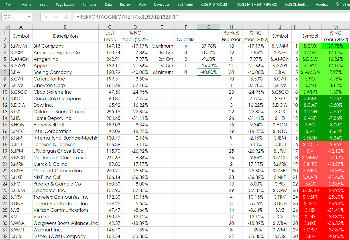
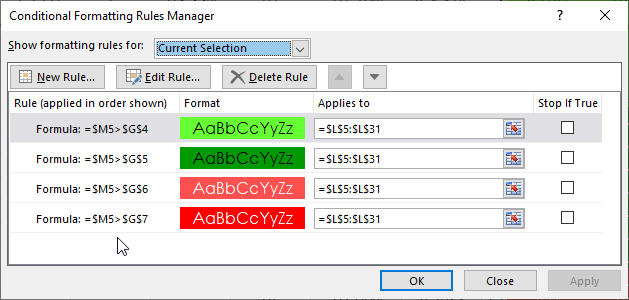
Next, the %NC values are ranked in column H. Columns L and M using VLOOKUP display the highest to the lowest values and their respective symbols. Finally, columns L and M have conditional formatting colors based on quartiles.
The downloadable sample spreadsheet on tab Sheet1 pulls in closing historical data using standard RTD calls and the AGGREGATE function to calculate a 20-bar moving average. In addition, the RSI oscillator values are pulled in and the maximum and minimum values are found using the AGGREGATE function.
One final note: On the Quartile tab copious use of Excel’s IFERROR functions are used for aesthetic purposes to display blank cells instead of #VALUE errors.
Requires CQG Integrated Client or CQG QTrader , and Excel 2010 or higher. Excel has to be installed on the local computer, not in the cloud.