The RTD function displayed in the title of the post includes the "@" sign. If you use the CQG RTD Toolkit installed on the Excel Ribbon when either CQG IC or QTrader are installed to pull in "Label" data the "@" sign is seen if you are running Excel 365 or higher.
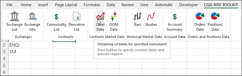
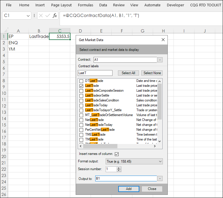
As shown below, selecting from the Label Data button using the CQG RTD Toolkit and then selecting Last Trade inserts the RTD function calling for the Last Trade using the symbol located in cell A1.
As shown in the above image the "@" sign is included in the function. This is done by Excel 365 or higher. The "@" sign is Excel's Implicit Intersection Operator. The "@" sign forces the function to only return one value. This is done as part of Excel 365's new Dynamic Array functions.
Prior to Excel 365 the Implicit Intersection Operator was functioning behind the scenes. If a function was entered and the returned output was an array then the formula had to be entered and then the key combination Ctrl + Shift + Enter was used and an array was returned.
Excel 365 offers Dynamic Arrays, and a special key combination is not required. Here is an example using Excel's FREQUENCY function to analyze the correlation between two markets. Excel's FREQUENCY function returns an array.
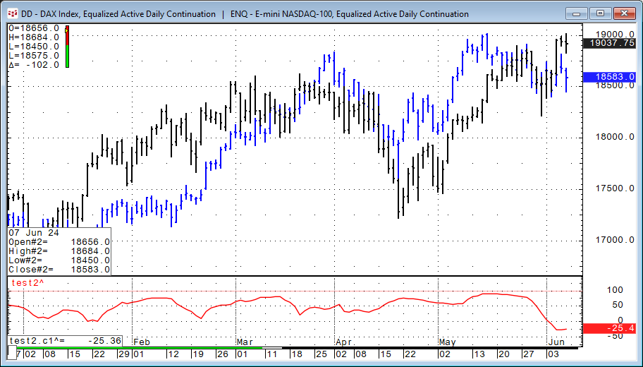
The chart above displays daily open, high, low, and close bars for the DAX Index (symbol: DD, blue bars) and overlayed is daily open, high, low, and close bars for the E-mini NASDAQ 100 Index (symbol: ENQ, black bars). The study is the rolling 20-day correlation between the two markets. One can see that the correlation is nearly always positive and sometimes nearing 100.
The image below shows the RTD formula for pulling in correlation data. Cell B6 has this formula and is copied down to cell B105:
=IFERROR(RTD("cqg.rtd",,"StudyData","Correlation("&$A$2&","&$B$2&","&$C$2&")", "Bar", "", "Close",$D$2,A6,,,,,"T")/100,NA())Cells A2 and B2 are the symbols, cell C2 is the lookback parameter for the correlation study, and cell D2 is the period, here "D" is for daily.
The FREQUENCY function calculates how often values occur within a range of values, and then returns a vertical array of numbers. The function requires the range of values, cells B6:B105 and a range of bins, cells C6:C26.
First, select cells D6:D26 and enter the formula:
=FREQUENCY(B6:B105,C6:C26)
And press the key combination Ctrl + Shift + Enter. The array populates with the counts in cells D6:D26.
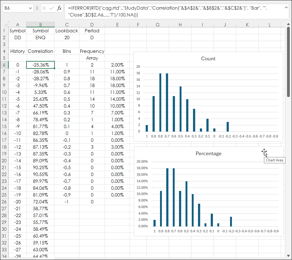
Now, the correlation values are viewed as a table of observations of the counts. Far better than viewing correlation as a line.
This next image shows how Excel 365 works with the FREQUENCY function.
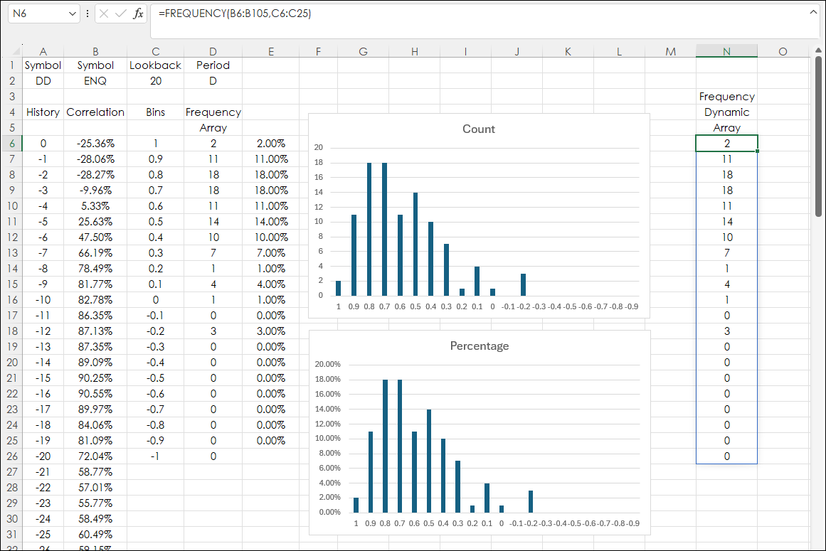
In cell N6 enter:
=FREQUENCY(B6:B105,C6:C26)
And hit Enter. And the entire array populates. If you select cell N6 the blue line appears indicating the array. Obviously, dynamic arrays are easier than the previous methods of working with arrays.
This post, Excel Combining SORTBY, CHOOSECOLS, and TAKE Functions, also discusses working with Dynamic Arrays.
The above spreadsheet is available for download.
Requires CQG Integrated Client or CQG QTrader, and Excel 365 or higher. Excel has to be installed on the local computer, not in the cloud.