The post "Excel Combining SORTBY, CHOOSECOLS, and TAKE Functions" discusses Excel 365's Dynamic Arrays and the concept of returned data automatically "spilling" into a collection of cells.
This post is an overview of this feature in Excel 365. The "Spill" feature is part of Excel 365 Dynamic Arrays. In earlier versions of Excel to return an array (more than one cell will display data) the user had to select the cells for the array, then enter the formula in the first cell and use key combination Ctrl+Shift+Enter.
Now, Excel 365 assumes that the data returned will be an array. In fact, to avoid returning an array the "@" sign is used right after the "=" in the RTD Formula.
A Dynamic Array is returned when using the FILTER function, which is used to find specific data in a table. For example, consider trading in the New York and London markets. One key aspect is they do not change from Daylight Savings Time to Standard Time on the same day. The United Kingdom changes back 1 hour at 2am on the last Sunday in October. The U.S. changes back 1 hour at 2am on the first Sunday of November. To know the dates of the two changes the FILTER function is used.
The sample Excel 365 offered at the bottom of this post lists the calendar days of a month in column B and column H starting with the Date in cell B3 and H3.
Cell B3 returns the date for October 1, 2024 (Change the year date for future years):
=DATE(2024,10,1)
Cell H3 returns the date for November 1, 2024 (Change the year date for future years):
=DATE(2024,11,1)
Then, cells B5 through B35 increase the dates by 1 day:
=B3
=B5+1
Etc.
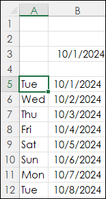
Then cells A5 through A35 converts the date to a day of the week:
=TEXT(B5,"DDD")
The result is the two columns have the days of the month and the dates:
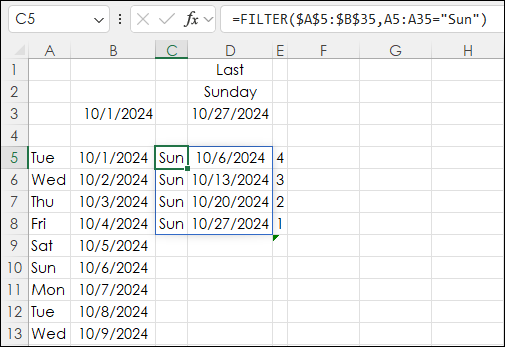
Next, the cells A5 through B35 are filtered for "Sun" in cell C5 ( the formula is entered in just cell C5) and Excel spills the data:
=FILTER($A$5:$B$35,A5:A35="Sun")
Selecting C5 and the light blue box appears indicating the "spilled" data (only cell C5 can be edited):
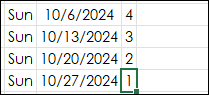
The RANK function is used in cells E5 through E9 to find the largest date:
=RANK(D5,$D$5:$D$9)
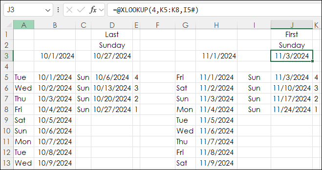
Then the XLOOKUP function is used to pull that date to a new cell:
=@XLOOKUP(1,E5:E9,D5:E9)
Notice the "@" right after the "=" sign. If the "@" was not used then the XLOOKUP function would have spilled to include the "1".
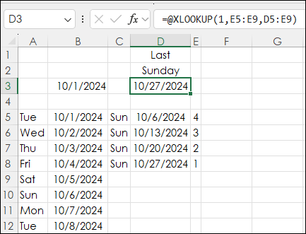
Also, notice that the range used above is cells E5:E9 and cells D5:D9. This is used because there are times when October will have five Sundays. The fact that October, 2024 only has four Sundays does not generate an error. This is a key feature of Dynamic Arrays.
These same steps were used to find the first Sunday in November, except the XLOOKUP looked for the number "4" in the ranking.
Excel 365's Dynamic Ranking is a very useful feature for pulling key data from a table. The dates pulled above can be used in a separate tab by linking the cells to the different tab.
Requirements: CQG Integrated Client or QTrader, and Excel 365 (locally installed, not in the Cloud) or more recent.