This post details using a nested XLOOKUP function to pull data from a matrix. The matrix displays the monthly percentage net change using a column for the symbols and a row for the months. The RTD formula for the monthly net percentage change is from this post: Basic Excel RTD Percent Net Change Formulas.
The RTD formula for the monthly percentage net change is:
=RTD("cqg.rtd",,"StudyData","S.MSFT", "PCB","BaseType=Index,Index=1", "Close", "M","0","all",,,,"T")As there is not an RTD formula for pulling percentage net change by month a method is used to pull individual monthly percent net change for each month.
Above, the RTD formula parameter for the current month is the "0". The "Index=1" parameter is to use the close from the previous month as the starting point. If we wanted the percent change from two months ago then the "Index=2" would be used and the one month percentage change from two months ago then "-1" would be used. For example:
=RTD("cqg.rtd",,"StudyData","S.MSFT", "PCB","BaseType=Index,Index=2", "Close", "M","-1","all",,,,"T")
As this post is being written in June then the Index is set to 1 and the lookback parameter is 0. For May the Index is set to 2 and the lookback parameter is -1. For April the Index is set to 3 and the lookback parameter is -2.
For Excel to automatically set the Index and Lookback parameters the Today() function is wrapped by the Month function, which returns an integer for the month. This function in cell S2 converts the month integer to a three letter month:
=IFS(MONTH(TODAY())=1,"Jan",MONTH(TODAY())=2,"Feb",MONTH(TODAY())=3,"Mar",MONTH(TODAY())=4,"Apr",MONTH(TODAY())=5,"May",MONTH(TODAY())=6,"Jun",MONTH(TODAY())=7,"Jul")
Row cells G3 to R3 uses the following formula copied across the row to determine the Index parameter for the month:
=IF($S$2=G2,1,IF(H3>0,H3+1,0))
Row cells G4 to R4 uses the following formula copied across the row to determine the Lookback parameter for the month:
=IF(G3=1,0,IF(G3=0,0,H4-1))
For the cells that are in the future the Index Parameters and Lookback Parameters are set to 0.
To calculate the Monthly Percentage Change, the Excel formula checks that if there is a "0" for the Index Parameter then a blank cell is returned. Otherwise, the RTD formula pulls the Monthly Percentage Change for the symbols in column B and uses the Index Parameter and the Lookback Parameter from the cells directly above.
This Excel formula is used for each of the columns:
=IF(G$3=0,"",IFERROR(RTD("cqg.rtd",,"StudyData",$B5, "PCB","BaseType=Index,Index="&G$3&"", "Close", "M",G$4,"all",,,,"T")/100,""))The Nested XLOOKUP function is used in cell U7:
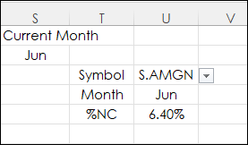
=XLOOKUP(U5,B5:B34,XLOOKUP(U6,G2:R2,G5:R34))
First, the function finds the symbol from the Dropdown List in cell U3 and the Month in the Dropdown List in cell U4 and returns the percent change for the month.
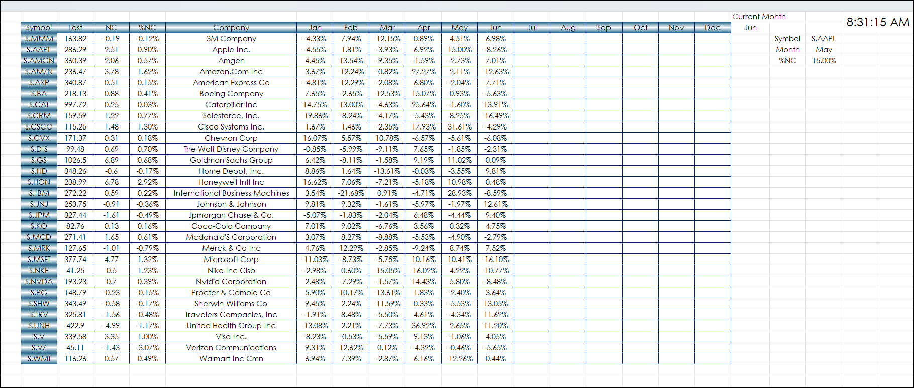
The full dashboard looks like this.
This post used a Nested XLOOKUP function to pull data from a matrix style monthly percentage net change quote display.
Requires CQG Integrated Client or CQG QTrader, data enablements for the NYSE and Nasdaq stocks, and Excel 2016 or more recent locally installed, not in the Cloud.