
This post is another example of using Excel functions and RTD calls to screen a large portfolio. The sample dashboard is the holdings of the S&P 500® Index (as of 7/20/2026). The screening is for market performance characteristics including the weekly, monthly, quarterly, and annual top ten percentage performers and bottom ten percentage performers. In addition, stocks with high volume trading, large net changes, and large Z-Scores are identified.
The dashboard has a Data Tab where all of the RTD formulas return the current market statistics.
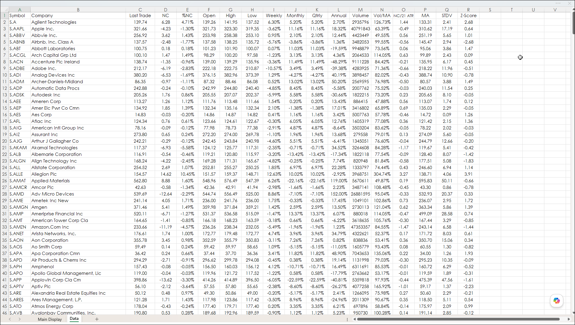
Here is a table of the RTD formulas used on the Data Tab.
Last Trade:
=RTD("cqg.rtd", ,"ContractData", A2, "LastTrade",, "T")Net Change of the Last Trade:
=RTD("cqg.rtd", ,"ContractData", A2, "NetLastTrade",, "T")Percent Change of the Net Change:
=IFERROR(RTD("cqg.rtd", ,"ContractData", A2, "PerCentNetLastTrade",, "T")/100,"")This Session's Open:
=RTD("cqg.rtd", ,"ContractData", A2, "Open",, "T")This Session's High:
=RTD("cqg.rtd", ,"ContractData", A2, "High",, "T")This Session's Low:
=RTD("cqg.rtd", ,"ContractData", A2, "Low",, "T")The Current Week's Percent Net Change (the IFERROR function is used because the returned value is divided by 100 to avoid seeing the #VALUE Error):
=IFERROR(RTD("cqg.rtd",,"StudyData", A2, "PCB","BaseType=Index,Index=1", "Close", "W","0","all",,,,"T")/100,"")The Current Month's Percent Net Change:
=IFERROR(RTD("cqg.rtd",,"StudyData", A2, "PCB","BaseType=Index,Index=1", "Close", "M","0","all",,,,"T")/100,"")The Current Quarter's Percent Net Change:
=IFERROR(RTD("cqg.rtd",,"StudyData", A2, "PCB","BaseType=Index,Index=1", "Close", "Q","0","all",,,,"T")/100,"")The Current Annual Percent Net Change:
=IFERROR(RTD("cqg.rtd",,"StudyData", A2, "PCB","BaseType=Index,Index=1", "Close", "A","0","all",,,,"T")/100,"")The Current Session's Volume:
=RTD("cqg.rtd", ,"ContractData", A2, "T_CVol",, "T")Yesterday's 21-day Moving Average of the Volume:
= IFERROR(M2/RTD("cqg.rtd",,"StudyData", $A2, "MA", "InputChoice=Vol,MAType=Sim,Period=21", "MA","D","-1","all",,,,"T"),"")The Current Session's Volume Ratio to Yesterday's 21-Day Moving Average of the Volume (yesterday's volume average is used as it is a fixed value):
=IFERROR(D2/RTD("cqg.rtd",,"StudyData","ATR("&A2&",MAType:=Sim,Period:=21)","Bar",, "Close", "D",,,,,,"T"),"")Today's 21-day Moving Average of the Closes:
= RTD("cqg.rtd",,"StudyData", $A2, "MA", "InputChoice=Close,MAType=Sim,Period=21", "MA","D",,"all",,,,"T")Today's 21-day Standard Deviation of the Closes:
= RTD("cqg.rtd",,"StudyData",$A2, "StdDev", "InputChoice=Close,Period1=21", "STDDEV","D",,"all",,,,"T")The STANDARIZE Function Calculates the Z-Score. (A returned Value of 2 indicates the current price is two standard deviations above of the 21- day mean of the closes):
=IFERROR(STANDARDIZE(C2,P2,Q2),"")
Main Display Tab
The Main Display tab uses Excel functions to scan the Data Tab for the best and worst performers for the current session.
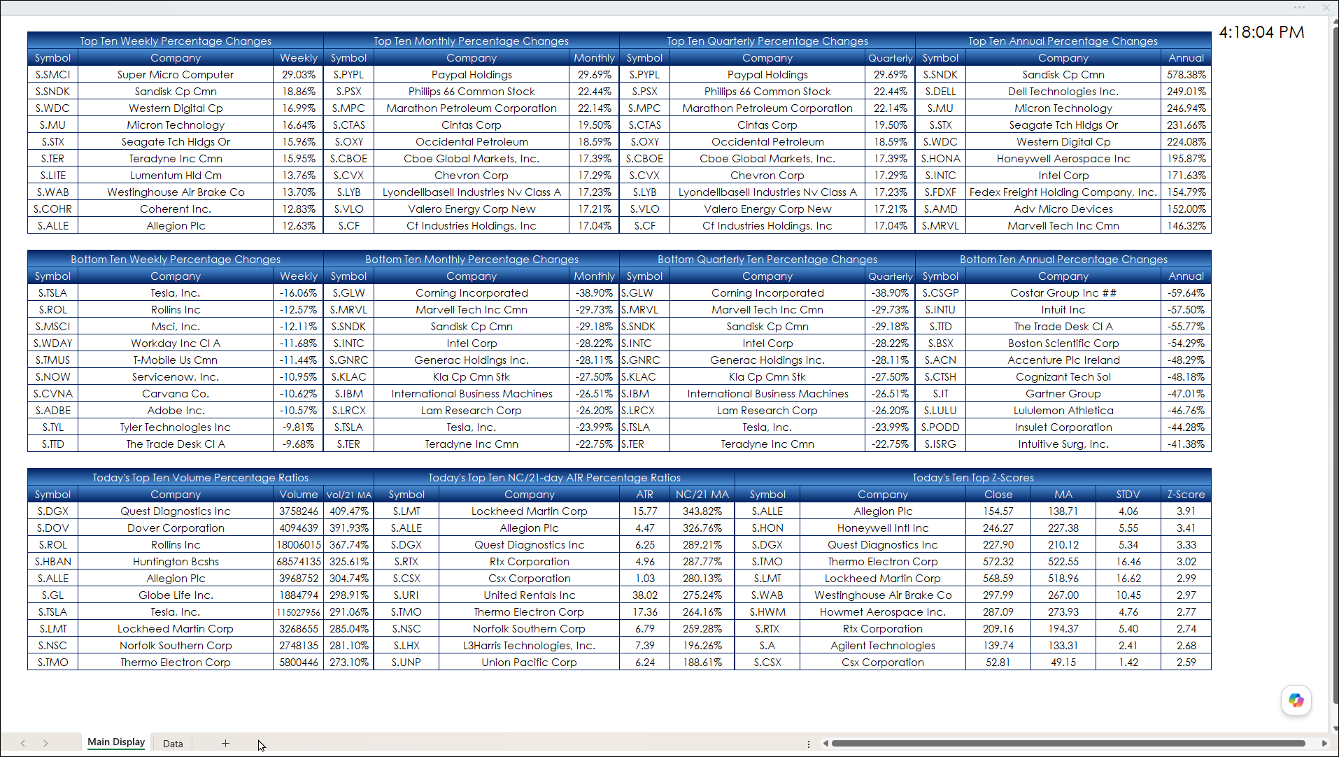
The top two blocks display the current top ten and bottom ten percent net change performers for the stocks in the S&P 500 using a weekly, monthly, quarterly, and annual view.
The blocks first pull in the symbols using Excel Functions from the Data Table. The Excel functions to pull in the symbols are nested. Here, used in cell B4 is the final version, which will be broken down to explain its use (when entered into cell B4 the Excel function "Spills" down to cell B13):
=CHOOSECOLS(TAKE(SORTBY(Data!A2:I504,Data!I2:I504,-1),10),1)
The "SORTBY" function is the starting point:
SORTBY(Data!A2:I504,Data!I2:I504,-1)
Above, the array is cells A2:I504 from the Data tab and sorted based on the data in cells I2:I504 in descending order (-1). Column A are the symbols and column I is Weekly Percent Change.
And only the top ten are returned by using the TAKE function:
TAKE(SORTBY(Data!A2:I504,Data!I2:I504,-1),10
And column A is the first column and what is needed are the symbols. The CHOOSECOLS function is used:
=CHOOSECOLS(TAKE(SORTBY(Data!A2:I504,Data!I2:I504,-1),10),1)
The above Excel function inserted into cell B4 pulls the first ten symbols sorted by the weekly percent change in descending order.
The next column is an RTD function pulling in the company name from the symbol in cell B4:
=PROPER(RTD("cqg.rtd", ,"ContractData",B4, "LongDescription",, "T"))The Weekly Percent Net change in cell C4 is pulling the data from the Data Tab:
=CHOOSECOLS(TAKE(SORTBY(Data!A2:I504,Data!I2:I504,-1),10),9)
The above Excel functions are used across the top block pulling percent net change based on the week, month, quarter and year from the Data Tab.
The next block is the bottom percent net change based on the week, month, quarter and year. The difference is the Excel function uses 1 instead of -1 in the SORTBY section:
=CHOOSECOLS(TAKE(SORTBY(Data!A2:I504,Data!I2:I504,1),10),1)
The same functions are used as in the Top Block except the 1 is used instead of -1 for ascending values.
The bottom block is pulling in studies.
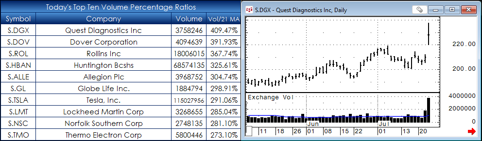
Today's Top Ten Volume Percentage Ratios
The volume percentage ratio compares today's volume to the previous session's 21-period of the volume. The previous moving average is used so today's volume is not included. The top ten ratios Excel function is entered into cell B30 and spills to cell B39.
The SORTBY function is modified to skip cells that do not have a value (Data!N2:N504<>""):
=CHOOSECOLS(TAKE(SORTBY(FILTER(Data!A2:N504,Data!N2:N504<>""),FILTER(Data!N2:N504,Data!N2:N504<>""),-1),10),1)
The RTD function for the company name is used in cell C30 to C39:
=PROPER(RTD("cqg.rtd", ,"ContractData",B30, "LongDescription",, "T"))The RTD function for today's volume is used in cell F30 to F39:
=RTD("cqg.rtd", ,"ContractData",B30, "T_CVol",, "T")The VLOOKUP Function entered into cell G30 to G39 pulls in the Volume Ratio from the Data tab using the symbols in column B:
=VLOOKUP(B30,Data!A2:N504,14,FALSE)
The table is shown below and a chart from CQG IC showing the price action and volume.
Today's Top Ten NC/21-day ATR Percentage Ratios
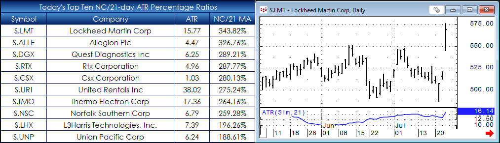
This block pulls in today's top ten Net Change/21-day Average True Range ratios. The top ten ratios Excel function is entered into cell H30 and spills to cell H39.
=CHOOSECOLS(TAKE(SORTBY(FILTER(Data!A2:O504,Data!O2:O504<>""),FILTER(Data!O2:O504,Data!O2:O504<>""),-1),10),1)
The RTD function for the company name is used in cells I30 to I39:
=IF(H30="","",PROPER(RTD("cqg.rtd", ,"ContractData",H30, "LongDescription",, "T")))The Average True Range RTD formula is entered into cells L30 to L39:
=IF(H30="","",RTD("cqg.rtd",,"StudyData","ATR("&H30&",MAType:=Sim,Period:=21)","Bar",, "Close", "D",,,,,,"T"))The VLOOKUP Function entered into cell M30 to M39 pulls in the NC/ATR Ratio from the Data tab using the symbols from column H:
=VLOOKUP(H30,Data!$A$2:$O$504,15,FALSE)
The table is shown below and a chart from CQG IC showing the price action and the ATR study.
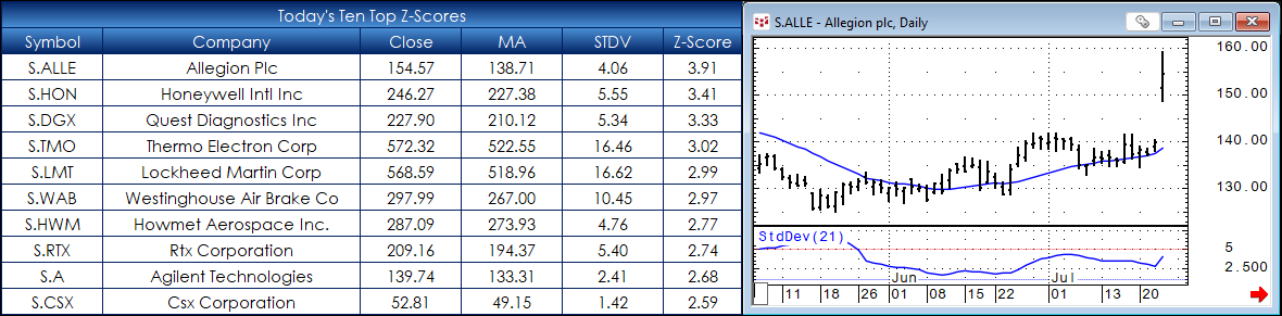
Today's Ten Top Z-Scores
A Z-Score is Z = (Close -Average)/Standard Deviation. If the Z-Score is 2 then the difference between the Close and the average is two standard deviations.
This block pulls in the top ten Z-Scores. Cell N30 has this function and spills down to cell N39:
=CHOOSECOLS(TAKE(SORTBY(FILTER(Data!A2:R504,Data!R2:R504<>""),FILTER(Data!R2:R504,Data!R2:R504<>""),-1),10),1)
This RTD function pulls in the company name and is entered into cells O30 to O39:
=PROPER(RTD("cqg.rtd", ,"ContractData",N30, "LongDescription",, "T"))This RTD formula entered into cells R30 to R39 pulls in the Last Trade using the symbols in cell N30 to cell N39:
=RTD("cqg.rtd", ,"ContractData",N30, "LastTrade",, "T")This VLOOKUP function entered into cells S30 to S39 pulls in the 21-peiod MA from the Data tab;
=VLOOKUP(N30,Data!$A$2:$P$504,16,FALSE)
This VLOOKUP function entered into cells T30 to T39 pulls in the 21-peiod Standard deviation from the Data tab:
=VLOOKUP(N30,Data!$A$2:$Q$504,17,FALSE)
This VLOOKUP function entered into cells U30 to U39 pulls in the Z-Score from the Data tab:
=VLOOKUP(N30,Data!$A$2:$R$504,18,FALSE)
The Z-Score table is shown below and a chart from CQG IC showing the price action and the Standard Deviation study.
This post illustrates the use of RTD formulas and Excel functions to monitor a large number of stocks and then highlighting the extreme movers. The downloadable Excel Dashboard can be modified on the Data Tab for symbols and studies.
This link is to a spreadsheet that lists RTD formulas for most studies and chart types.
Requires CQG Integrated Client or CQG QTrader, data enablements for the NYSE and Nasdaq stocks, and Excel 2016 or more recent locally installed, not in the Cloud.