
Excel has some very useful functions for screening market performance data and filtering large amounts of data to highlight particular user defined results for further analysis.
This post offers a downloadable Excel dashboard that uses Excel's FILTER and CHOOSECOLS functions that screens data and returns a list based on the user defined events.
For illustrative purposes the companies in the Dow Jones Industrial Average (DJIA) is the portfolio analyzed. The value of using these functions would be shown if the portfolio was larger, such as the 500+ companies in the S&P 500.
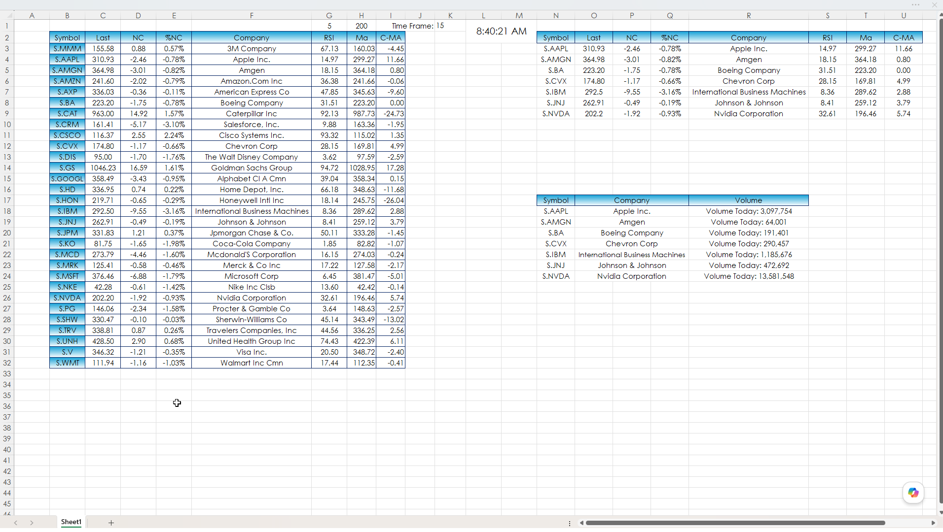
This image is the portfolio with two studies: Relative Strength Index (RSI) and a moving average.
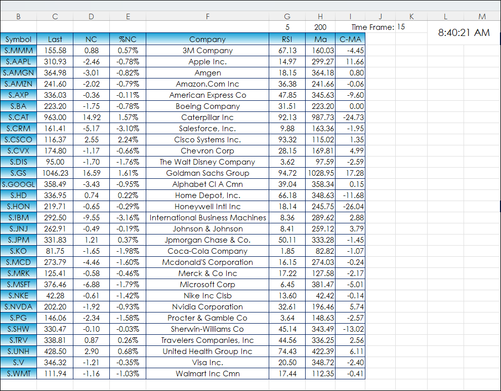
Column G is the RTD formula for pulling the RSI study values for each stock:
=RTD("cqg.rtd",,"StudyData",B3,"RSI","Period="&$G$1&",InputChoice=Close","RSI",$K$1,"0","all","","","False","T","ExcelInterval","")The lookback period is pulled from cell $G$1. The time frame is pulled from cell $K$1
Column H is the RTD formula for pulling the Moving Average study values for each stock:
=RTD("cqg.rtd",,"StudyData",B3,"MA","MAType=Sim,Period="&$H$1&",InputChoice=Close","MA",$K$1,"0","all","","","False","T","ExcelInterval","")The lookback period is pulled from cell $H$1. The time frame is pulled from cell $K$1
Column I calculates the difference between the current Last Trade and the moving average:
=C3-H3
A simple concept is if the stock price is above the 200 period moving average (the trend is up) and the 5-period RSI is below 38 then the stock is pulling back against the trend.
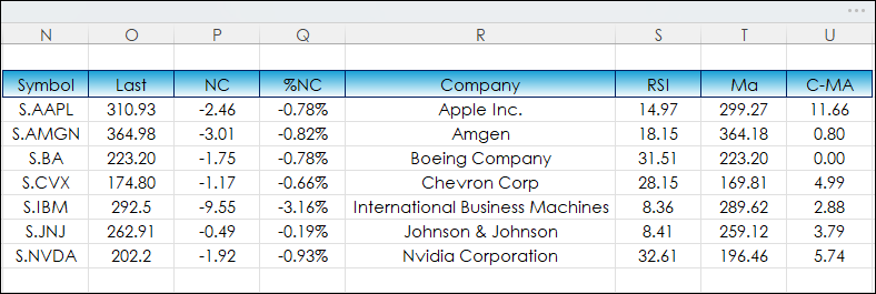
To see the list of stocks currently in that situation the FILTER function is used in cell N3:
=IFERROR(FILTER(B3:I32,(G3:G32<38)*(I3:I32>0)),"")
The IFERROR function is used because if none of the stocks meet the criteria an error is generated. This function replaces the error with a blank cell.
The FILTER function is screening cells G3 to I32 for two conditions: The RSI is below 38 (cells G3:G32) and the last trade is above the moving average (cells I3:I32).
The “*” is “And”.
The FILTER function spills a table of the companies meeting the two criteria:
With this information the CHOOSECOLS function is used to pull the symbols meeting the two criteria and displays the list of symbols starting with cell N18:
=CHOOSECOLS(FILTER(N3:X12,N3:N12<>""),1)
The CHOOSECOLS function is pulling the first column in the table cells N3:X12 (the symbols). The CHOOSECOLS function will return “0” if there is not a symbol. To avoid this the FILTER function is used to only pull symbols when there is a symbol (N3:N12<>"").
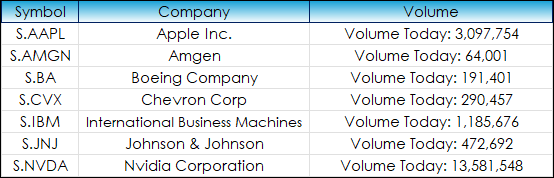
With that symbol list more data can be called for more analysis. A simple example: The name of the company and the current volume.
=IF(N18="","",PROPER(RTD("cqg.rtd", ,"ContractData",N18, "LongDescription",, "T")))=IF(N18="","","Volume Today: "&TEXT(RTD("cqg.rtd",,"ContractData",N18,"T_CVol",,"T"),"#,###"))The full dashboard:
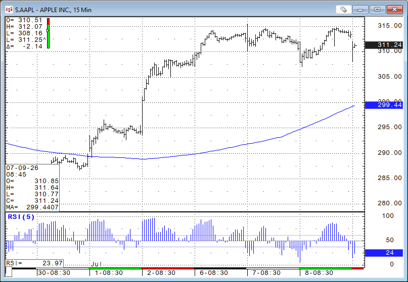
This post was created while the markets were open, consequently some market and study values may not match image to image.
The FILTER functions spill tables. If a larger portfolio is used the FILTER functions may need to be moved to avoid running into each other.
This post was an example of using Excel functions to screen for user defined conditions.
Requires CQG Integrated Client or CQG QTrader, data enablements for the NYSE and Nasdaq stocks, and Excel 2016 or more recent locally installed, not in the Cloud.