A post titled "Excel Indirect Function and More" was published on February 22, 2022, that detailed using Excel's INDIRECT function, as well as details to automatically format cells for displaying price quotes with the correct number of decimal places.
In this post the use of the INDIRECT function as a way to dynamically set the "Table Array" for the VLOOKUP function.
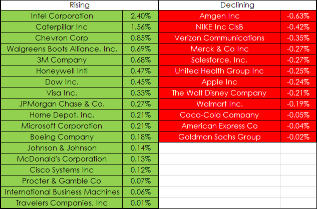
For example, consider designing a table with two sets of groups: One group displays the descriptions and net percentage change of the thirty stocks comprising the Dow Jones Industrial Average that are positive for the session. The second group displays the descriptions and net percentage change of the thirty stocks that are negative for the session.
The process in Excel requires four steps:
- Pull in market data using RTD calls.
- Rank the data using an Excel function.
- Sort the ranked data from highest to lowest using an Excel function.
- Resort the data into two groups: Rising and declining.
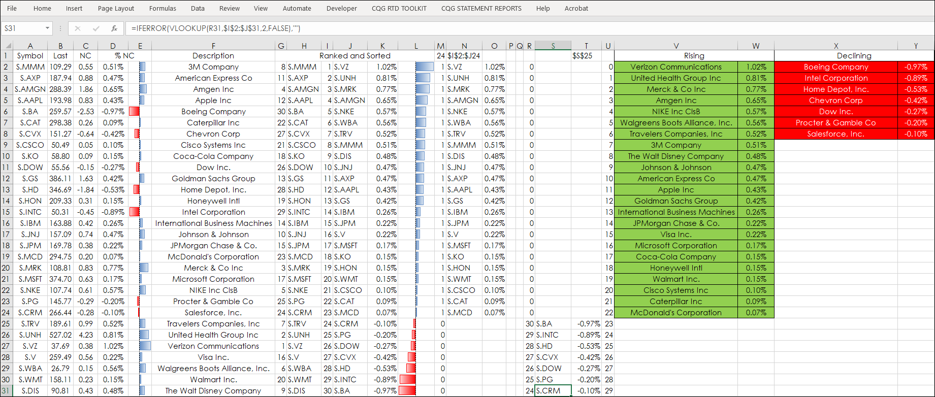
The symbols are in column A. Columns B through F pull in the market data using RTD calls. Below are the RTD calls for columns B through F. Column D and E are duplicates because column E has the data bars conditions applied to it. Also, the IFERROR function is employed to display blank cells.
=RTD("cqg.rtd", ,"ContractData", A2, "LastTrade",, "T")
=RTD("cqg.rtd", ,"ContractData", A2, "NetLastTradeToday",, "T")
=IFERROR(RTD("cqg.rtd", ,"ContractData", A2, "PerCentNetLastTrade",, "T")/100,"")
=IFERROR(RTD("cqg.rtd", ,"ContractData", A2, "PerCentNetLastTrade",, "T")/100,"")
=RTD("cqg.rtd", ,"ContractData", A2, "LongDescription",, "T")
Columns G through L rank the markets' performance by percentage net change and sort the markets by highest percentage net change to lowest.
Column G ranks the markets' performance by percentage net change. The Excel Rank function will assign ties the same value. So, you could see 7, 1, 3, 5, 3, 2, 6 for the scores. And using VLOOKUP to sort the scores will return an error due to the duplicated value in the table array. The solution is to use the COUNTIF function with the RANK function and ties are automatically avoided.
Column G:
=IFERROR(RANK($D2,$D$2:$D$31)+COUNTIF($D2:$D2,D2)-1,"")
Column H pulls the symbols from column A: =A2
Column I is simply the numbers 1 through 30 for the VLOOKUP function to use for the lookup value from the table array columns G and H.
Column J is the VLOOKUP function returning the sorted ranked symbols from column H:
=IFERROR(VLOOKUP(I2,$G$2:$H$31,2,FALSE),"")
Columns K and L pull the percentage net change using the ranked and sorted symbols from column J. Column L has Excel's data bars conditions applied to it.
=IFERROR(RTD("cqg.rtd", ,"ContractData", J2, "PerCentNetLastTrade",, "T")/100,"")
Columns M through X separate the 30 stocks net percentage change into two groups: One group is the positive net percentage change, and one group is the negative net percentage change.
VLOOKUP is used but the "Table Array" parameter will use Excel's INDIRECT function so the Table Array parameter will dynamically change throughout the market session. To start, Column M determines if the net change from column K is positive or negative. In cell M2 this formula is used and copied down:
=IF(K2>=0,1,0)
Then, cell M1 sums the number of positive scores and adds 1 as this sum is used as the end row number for the Table Array in the VLOOKUP function:
=SUM(M2:M31)+1
In cell N1 the parameter for the "Table Array" for the VLOOKUP is created:
="$I$2:$J"&M1
Cell N2 has the VLOOKUP function (and is copied down) that uses INDIRECT as the second parameter:
=IFERROR(VLOOKUP(I2,INDIRECT($N$1),2,FALSE),"")
In this case above, the
VLOOKUP(I2,INDIRECT($N$1),2,FALSE),"")
converts to
VLOOKUP(I2, $I$2:$J23,2,FALSE),"")
And, if the number of positive net percentage changes expands or contracts, then so will the "Table Array" parameter.
The tallying of the number of stocks with a negative net percentage is a little more complicated. In column R (column Q is empty) cell R2 has this formula:
=IF(K2>=0,0,30)
This formula above is checking that K2 is positive and if it is then a 0 is returned, and if not True then 30 is returned. The reason 30 is used is there are 30 stocks in the DJIA, then if K2 is negative then all of the stocks are negative.
Cell R3 has this formula and is copied down:
=IF(K3>=0,0,IF(R2=0,30,R2-1))
It is checking if K3 is not postive, then it is checking if the cell directly above is 0, then return 30, otherwise subtract 1 from the cell above.
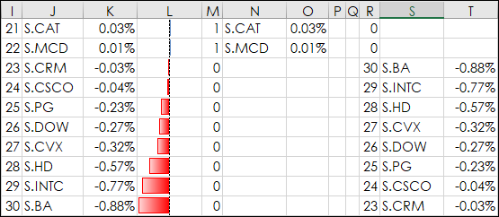
The net result is the sorted ranked symbols in columns I and J above are reversed and displayed in columns R and S.
Column V is the rising column and in cell V2 the long description is pulled using the symbol from cell N2 and this is copied down.
=IF(N2="","",IF(M2=0,"",RTD("cqg.rtd", ,"ContractData", N2, "LongDescription",, "T")))
And the net percentage change is pulled from column O and copied down:
=O2
The declining stocks use the cell with the first 30 to start found by using the MATCH function.
In Cell T1 the MATCH function is used:
="$S$"&MATCH(30,R2:R31,0)+1
This returns the row number of the cell with the first 30 and is merged with "$S$" for the start of the declining group.
For pulling the long description:
=(INDIRECT(T1)=0,"",RTD("cqg.rtd", ,"ContractData", INDIRECT(T1), "LongDescription",, "T")),"")
The net percentage change checks that there is a value for the long description and if yes, uses T1:
=IF(X2="","",RTD("cqg.rtd", ,"ContractData", INDIRECT(T1), "PerCentNetLastTrade",, "T")/100)
The next set of cells use cell T1 plus a counter that adds an integer brought from column U. But, cell T1 first has to be separated and uses the TEXTAFTER function (requires Excel 365) and then merges in the new integer:
RTD("cqg.rtd",,"ContractData",INDIRECT("$S$"&TEXTAFTER($T$1,"$",2)+U3),"LongDescription",,"T"))
The result is, for example, $S$23 becomes $S$24.
But first, there needs to be a check for if the cell returns a value.
=IF(INDIRECT("$S$"&TEXTAFTER($T$1,"$",2)+U3)=0,"",RTD("cqg.rtd",,"ContractData",INDIRECT("$S$"&TEXTAFTER($T$1,"$",2)+U3),"LongDescription",,"T"))
For the actual net percentage change column, the formula is entered in cell Y2 and copied down:
=IF(X2="","",RTD("cqg.rtd", ,"ContractData", INDIRECT(T1), "PerCentNetLastTrade",, "T")/100)
The two sets of data are color condition: Green for rising and red for declining. The IFERROR function was used throughout the spreadsheet.
This post detailed how you can use the INDIRECT function within the VLOOKUP function to create dynamic "Table Arrays" to build a more sophisticated dashboard. The sample downloadable Excel spreadsheet is not locked.
Requirements: CQG Integrated Client or QTrader, and Excel 365 (locally installed, not in the Cloud) or more recent.