Microsoft Excel 365 introduced the LET Function. Excel 365 or Excel 2016 introduced the IFS function. This post details using the two functions for tracking the performance of the stocks comprising the Dow Jones Industrial Average.
Using the LET function enables you to assign names to calculation results and supports up to 126 names and calculations. For example (from the Microsoft Help file):
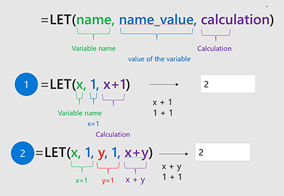
You can assign a name , a name value or calculation.
The downloadable Excel sample uses the LET function to assign one to three icons (▲, ▲ ▲, ▲ ▲ ▲) based on the ranked percentage difference between two moving averages.
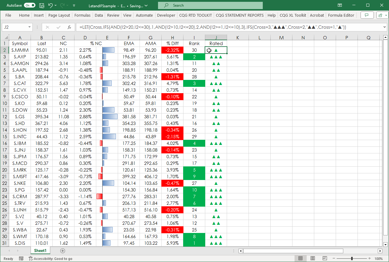
Column F is using RTD to pull in the Exponential Moving Average value with a smoothing constant period of 28 using the symbol in cell D2.
=RTD("cqg.rtd",,"StudyData","MA("&A2&",MAType:=Exp,Period:=28,InputChoice:=Close)", "Bar", "", "Close","D","0",,,,,"T")Column G is using RTD to pull in the Adaptive Moving Average value with smoothing constants of ERPeriod:=10, FastPeriod:=2, SlowPeriod:=30, using the symbol in cell D2.
=RTD("cqg.rtd",,"StudyData","AMA("&A2&",ERPeriod:=10,FastPeriod:=2,SlowPeriod:=30,InputChoice:=Close)", "Bar", "", "Close","D","0",,,,,"T")In column H the percentage difference between the two moving averages is calculated and the cells are formatted as percentages.
=(G2-F2)/F2
The percentage difference is ranked in column I and includes the COUNTIF function to avoid ties.
=RANK(H2,$H$2:$H$31,0)+COUNTIF($H$2:H2,H2)-1
At the time of this writing Walt Disney (Symbol: DIS) was the highest ranked performing stock. The blue line is the AMA, and the green line is the EMA.
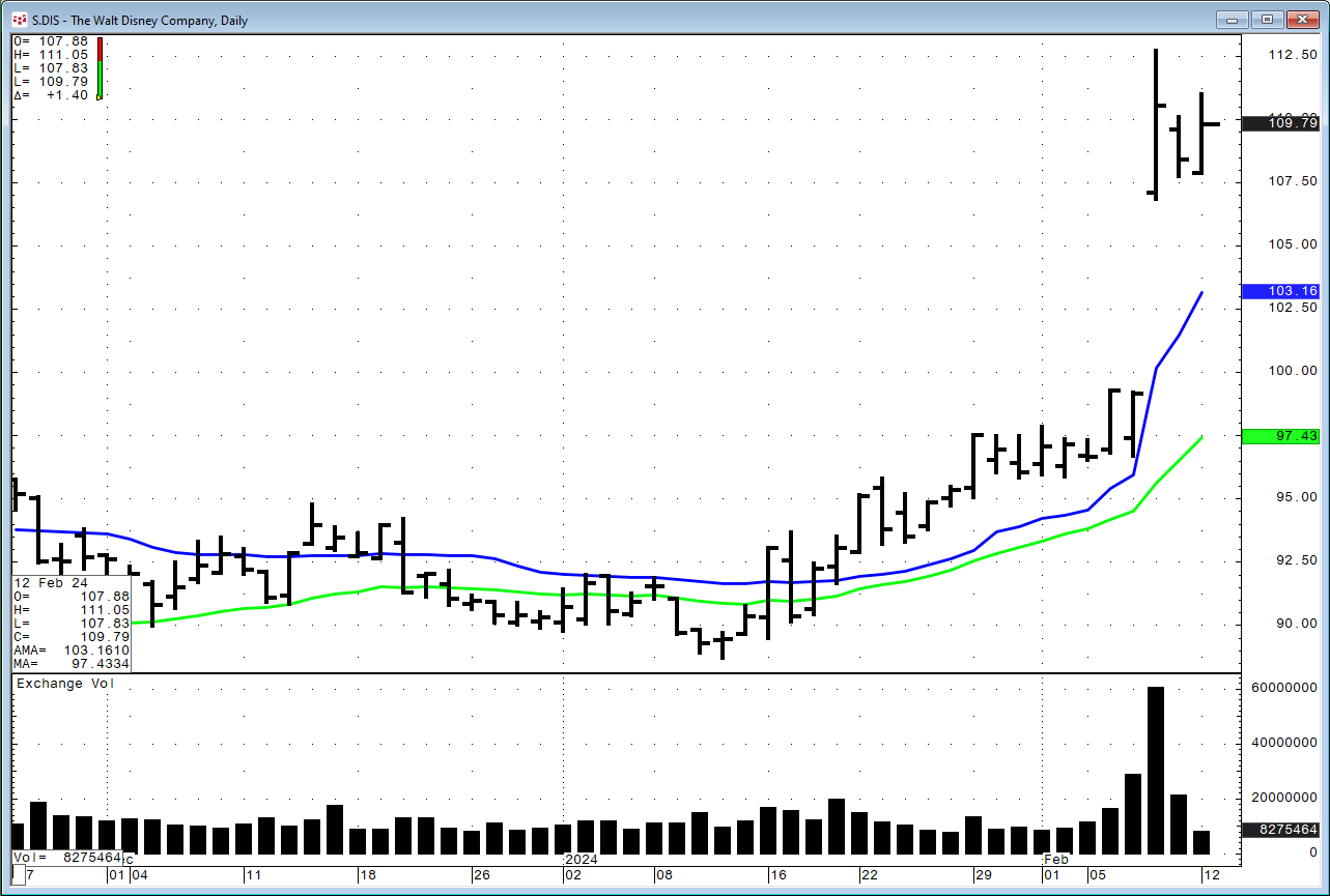
While 3M Company (Symbol: MMM) was the lowest ranked performing stock.

Column J is using the LET function to display one of three icons depending on the ranked percentage values placement in a bin with 1 being the top and 30 being the bottom: 1 up to and including 10 (▲ ▲ ▲), greater than 10 up to and including 20 (▲ ▲), and greater than 20 and up to and including 30 (▲).
In the LET function the name of the variable is Cross. The calculation is using the IFS function to determine which of the three bins the ranked percentage value falls in. The IFS function was covered in this post.
Note: The IFS function will check for each condition to be true and when it finds the first one it stops the review process. For example, let’s say the condition is checking for a value greater than 1, then greater than 5, and then greater than 10 in this order, i.e. IFS(V>1, a, V>5,b, V>10, C). If V is 15 then a is returned because V is greater than 1.
The Excel functions in column J:
=LET(Cross,IFS(AND(I2>20,I2<=30),1,AND(I2>10,I2<=20),2,AND(I2>=1,I2<=10),3),IFS(Cross=3,"▲▲▲",Cross=2,"▲▲",Cross=1,"▲"))
In addition, Column H (% Diff) is highlighted in red to indicate negative values. Column I (% Rank) is highlighted with green cells those cells in the top 10. Finally, the LET function can be very useful for data visualization of conditions. This post details how to easily find the appropriate RTD formula for studies.
Requirements: CQG Integrated Client or QTrader, and Excel 365 (locally installed, not in the Cloud) or more recent.