Excel 365 offers the LARGE and XLOOKUP functions. This post details using both for tracking market performance.
The image below is a table from Excel where the data presented are percent net change of monthly bars for the last twelve months.

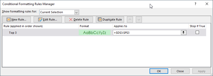
In addition, the data has conditional formatting highlighting the top 3 months for each symbol (row). The condition applies a green color to the background.

Notice that the same color is applied to the backgrounds of the top 3 performers.
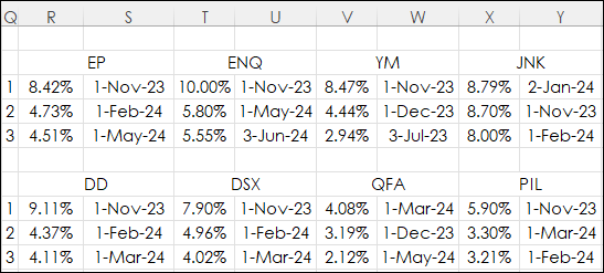
An additional table can be produced that displays the top 3 performers and the associated months.

The top three performers can be pulled from each market using Excel 365’s LARGE function:
=LARGE($D$3:$O$3,$Q3)
The LARGE function has two parameters: An array, which are the cells D3:O3 in the first image, and the parameter K, which is the position (from the largest) in the array or cell range of data to return. In this case above, it is cell Q3, and the value is 1 or first. The LARGE function is used for each row and builds a block of performance from 1 to 3 for each symbol.
Next, the month that represents each of the top three performers. CQG uses the starting date for a monthly chart. For that data the XLOOKUP function is used:
=XLOOKUP(R3,$D$3:$O$3,$D$2:$O$2)
THE XLOOKUP function looks for the value in cell R3 in rows D3:O3 and returns the associated value in the Date row (D2:O2). More details regarding using the XLOOKUP function are available in this post.
Excel 365’s LARGE function alleviates the requirement to perform any ranking of the data. The XLOOKUP function is an improvement over VLOOKUP. The downloadable Excel sample is the same as the images in this post.
Requirements: CQG Integrated Client or QTrader, and Excel 365 (locally installed, not in the Cloud) or more recent.