This posts details the use of two Excel functions: AVERAGEIFS and COUNTIFS. To start, a simple example of using the AVERAGEIFS function is presented.
In the image below column cells A2:A10 are simply labels A, B, and C.
Cells B2:B10 are values. Then cell D2 has the standard AVERAGE function for cells B2:B4.
=AVERAGE(B2:B4)
Cell D3 has the standard AVERAGE function for cells B5:B7.
=AVERAGE(B5:B7)
And cell D4 has the standard AVERAGE function for cells B8:B10.
=AVERAGE(B8:B10)
Cells E2:E4 use the AVERAGEIFS function. This function returns the average of all cells that meet one or more multiple criteria.
The parameters are:
- Average range: Required. One or more cells to average, including numbers or names, arrays, or references that contain numbers.
- Criteria range1, criteria range2,...
- Criteria range1 is required, subsequent criteria ranges are optional. 1 to 127 ranges in which to evaluate the associated criteria.
- Criteria1, criteria2, ...
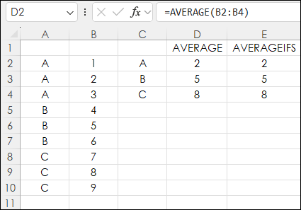
Cell E2 is calculating the Average of cells $B$2:$B$10 using the criteria range in cells $A$2:$A$10 and the criteria is "A" found in cell C2.
=AVERAGEIFS($B$2:$B$10,$A$2:$A$10,C2)
The returned value is 2 which matches the value in cell D2.
Cells E3 and E4 employs these two functions respectfully:
=AVERAGEIFS($B$2:$B$10,$A$2:$A$10,C3)
=AVERAGEIFS($B$2:$B$10,$A$2:$A$10,C4)
Cells E3 and E4 match cells D3 and D4.
Notice the only difference in these three Excel functions is the final parameter for the criteria in cells C2, C3, and C4.
The Average function in cell D2 had to be set to a specific range of B2:B4, and then the Average function in cell D3 had to use a new range (B5:B7) and the Average function in cell C3 had to use a new range (B8:B10).
Using the AVERAGEIFS function used the same cell range, the same criteria range, and a different criteria reference. The AVERAGEIFS function is a simpler application.
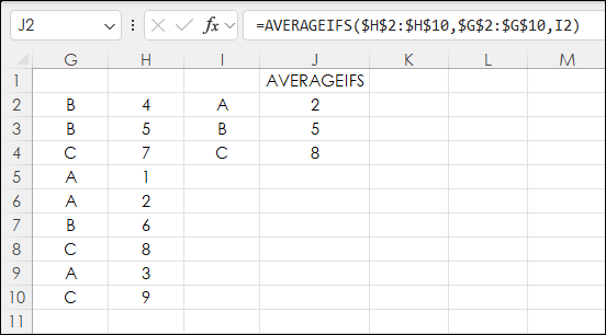
One final example in the image below is the letters and the appropriate values are scrambled in column G with the values in column H and the AVERAGEIFS function returns the correct averages in cells J2, J3, and J4.
Tip: To add the two $ to the Excel function to lock the cell references for copying and pasting simply place the cursor between the H and the 2 and hit the F4 key.
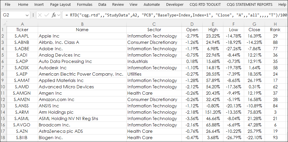
Next, the AVERAGEIFS function is used to determine the annual percent net change of stocks by sectors in the NASDAQ 100 index. The downloadable sample at the end of the post has an NDX tab.
Column A are the Ticker symbols in alphabetical order. Column B is the name of the company, column C is the sector the company is assigned to. Columns D, E, F, and G are the annual percent change for the open, high, low, and close. Column H is the current rank based on the close from column G.
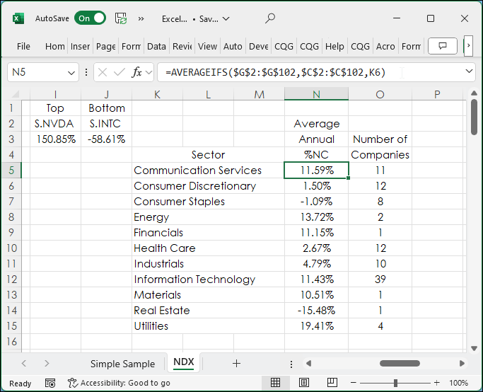
In the image below, this Excel formula is used in cell N5 and copied down to N15:
=AVERAGEIFS($G$2:$G$102,$C$2:$C$102,K5)
The "Average" range is: $G$2:$G$102
The "Criteria" range is: $C$2:$C$102
The "Criteria" is: K5
Column O uses the COUNTIFS function in cell O5 and copied down to O15 and returns the number of companies in each sector:
=COUNTIFS($C$2:$C$102,K5)
Cell I2 using XLOOKUP reviews the Ranked column (H2:H102) and finds the symbol in column A2:A102 for the top ranked stock.
=XLOOKUP(1,H2:H102,A2:A102)
Cell I3 using XLOOKUP reviews the Symbol column (A2:A102) and finds the annual percent change in column G2:G102 for the top ranked stock.
=XLOOKUP(I2,A2:A102,G2:G102)
The same process is used in cells J2 and J3 to find the bottom ranked stock.
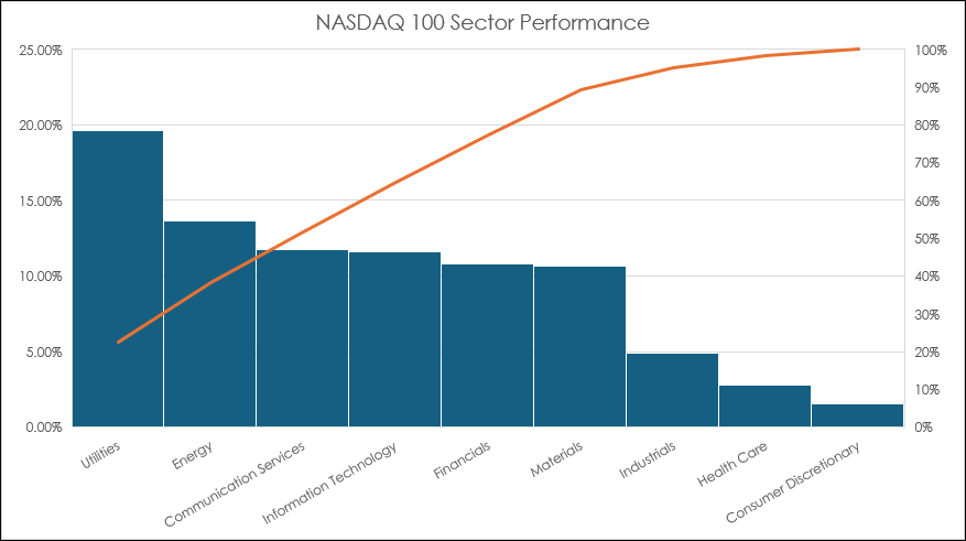
This next image is a Pareto Chart. A Pareto chart is a histogram chart automatically displaying columns sorted in a descending order and a line representing the cumulative total percentage. Pareto charts highlight the largest factors in a data set.
In the image below the Utilities sector is up the most for the year at time of this writing. There are just four companies in the Utilities sector. There are only two companies in the Energy sector.
The AVERAGEIFS function is one of a number of functions that are useful for analyzing a large table of values. The use of the Criteria parameter leads to a more efficient function than manually selecting individual ranges for calculating an average.
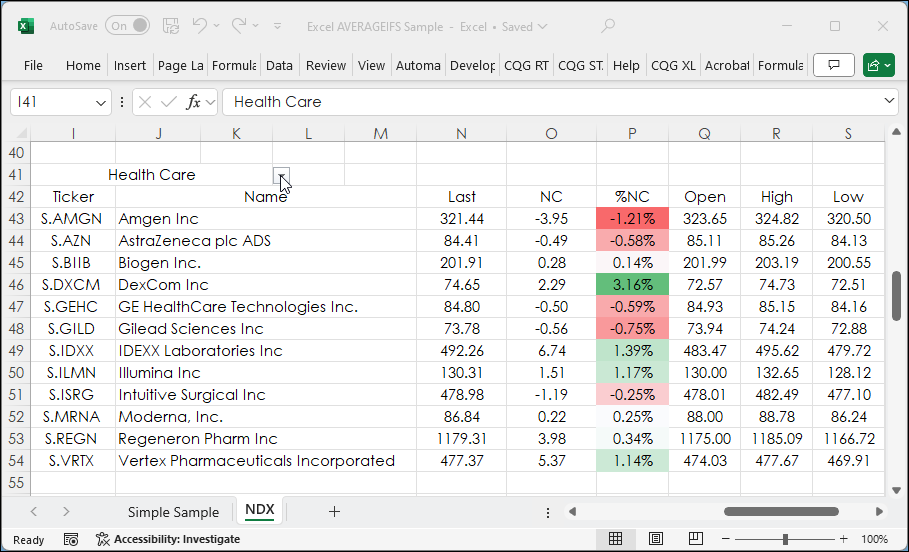
The spreadsheet also includes a drop down list of the sectors in cell I41. Choose one and using the FILTER function the companies in the specified sector will populate starting in cell I43 the ticker.
=FILTER($A$2:$A$102,$C$2:$C$102=I41)
This list of tickers per sector is not static and will expand or contract depending on the selected sector. To avoid RTD errors when blank cells are at the bottom of the ticker list an If Then statement is used.
=IF(I43="","",RTD("cqg.rtd", ,"ContractData", I43, "LongDescription",, "T"))The RTD formulas return the Description, Last Trade, Net Change, Percentage Net Change, Open, High, Low, and Close are pulled in. The Percentage Net Change column is heat mapped.
The AVERAGEIFS function is one of a number of functions that are useful for analyzing a large table of values. The use of the Criteria parameter leads to a more efficient function than manually selecting individual ranges for calculating an average.
Excel Functions used:
- AVERAGEIFS(), available in Excel 2007
- RANK ()+COUNTIF(), available in Excel 2007
- COUNTIFS(), available in Excel 2007
- XLOOKUP(), available in Excel 365 and 2021
- FILTER(), available in Excel 365 and 2021
- Pareto chart, available in Excel 2016
Requires CQG Integrated Client or CQG QTrader, and recommended Excel 365 or Excel 2021 or higher. Excel has to be installed on the local computer, not in the cloud.