Microsoft Excel 365 offers the TRIMRANGE function which excludes all empty rows and/or columns from the outer edges of a range or array. This post details how this function is useful for designing a template for an Excel Dashboard that allows for different sets of symbols.
A typical Excel market dashboard must account for the number of symbols as a starting point. The dashboard can take the symbols, for example, and display a ranked percent net change column.
However, adding more symbols necessitates modifying formulas to account for the increased number of symbols. The TRIMRANGE function removes that issue.
The TRIMRANGE function uses two parameters. For example:
=TRIMRANGE(range,[trim_rows])
Range is the cells to be trimmed, such as cells C1:C25.
The second parameter sets which rows should be trimmed:
0 - None
1 - Trims leading blank rows
2 - Trims trailing blank rows
3 - Trims both leading and trailing blank rows (default)
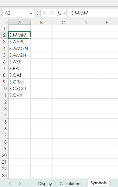
Here is an example. First, consider a dashboard that has a Symbols tab, a Calculations tab, and a Display tab.
In the image below five stock symbols are entered on the Symbols tab.
On the Calculations tab the A column is linked to Column A from the Symbols tab (=Symbols!A:A).
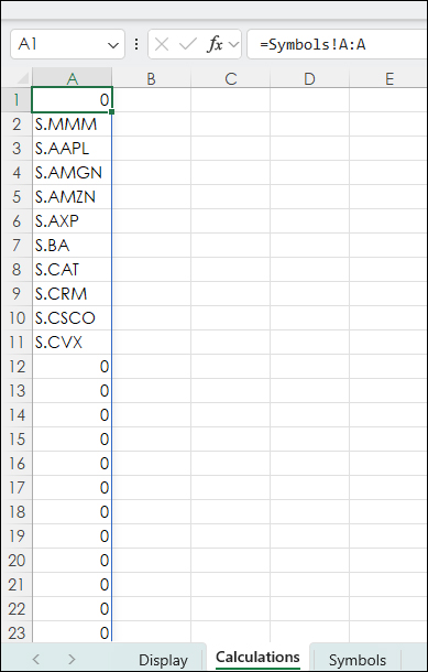
Above, we see that blank cells from the Symbols tab are filled in with "0"s.
The use of the TRIMRANGE function to clean up the data is next. Three parameters for trimming are presented.
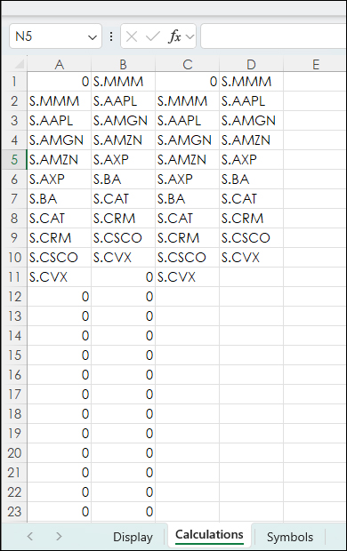
Above, column B is using:
=TRIMRANGE(Symbols!A:A,1)
The "1" trims leading blank rows.
Column C is using:
=TRIMRANGE(Symbols!A:A,2)
The "2" trims trailing blank rows.
Column D is using:
=TRIMRANGE(Symbols!A:A,3)
The "3" trims both leading and trailing blank rows and is the default.
Column A now has this function:
=TRIMRANGE(Symbols!A:A)
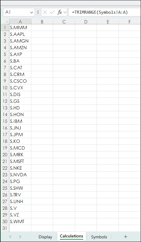
The Symbols tab was expanded to 30 symbols (the DJIA) and the Calculations tab automatically displays the 30 with no blank cells. There is a second method to use the TRIMRANGE function: Trim References (aka Trim Refs).
A Trim Ref can be used to achieve the same functionality as TRIMRANGE by replacing the range's colon ":" with one of the three Trim Ref types described below.
Trim All (.:.)
Trim Trailing (:.)
Trim Leading (.:)
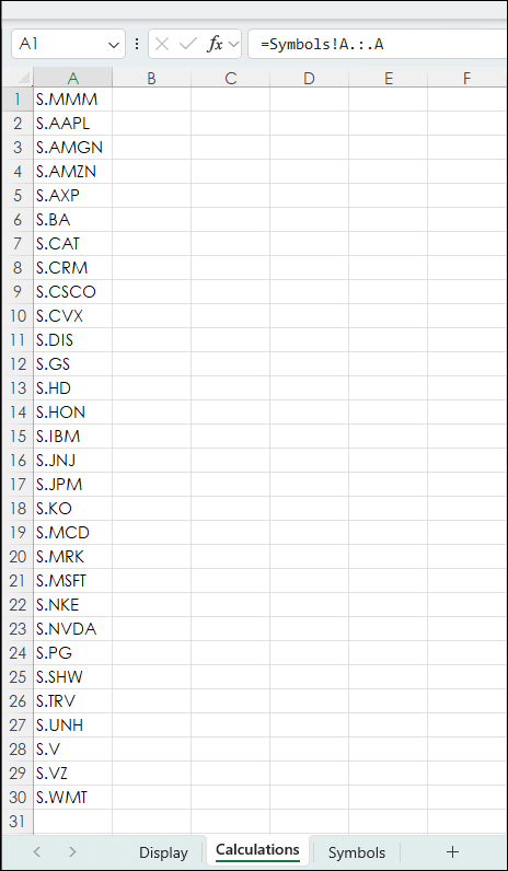
Above, in cell A1 the Trim Ref version is used:
=Symbols!A.:.A
Now, whatever number of symbols entered in the Symbols tab is automatically pulled to the Calculations tab without blank spaces.
The Calculations tab is where Excel and RTD formulas are used as the basis for the Display tab.
First, the data will be sorted by percentage net change for the day. This will also be used on the Display tab. An IF THEN statement is used. If cells in column A are blank, then the formula displays a blank cell.
=IF(A1="","",IFERROR(RTD("cqg.rtd",,"ContractData",A1,"PerCentNetLastTrade",,"T")/100,""))The IFERROR function is used because the value is divided by 100 for a percentage value. Before the opening, the data cache is cleared, and this avoids seeing #VALUE errors before trading begins.
All of the following formulas are copied down to row 200 on the Calculations tab. Column C and D uses Excel's "SORT" function. The link is to a post detailing this function.
=SORT(A1:INDIRECT("B"&COUNTA(A:A)),2,-1)The SORT function is analyzing cells A1 to cells in column "B" merged with the number of cells with values (COUNTA) in column A, sorted by the values in column B in descending order (-1).
Columns C and D are the ranked values and return the symbol and percentage net change.
Column E is the Long Description using symbols from column C:
=IF(A1="","",RTD("cqg.rtd",,"ContractData",C1,"LongDescription",,"T"))Column F is Last Trade:
=IF(A1="","",RTD("cqg.rtd",,"ContractData",C1,"LastTrade",,"T"))Column G is Net Last Trade:
=IF(A1="","",RTD("cqg.rtd",,"ContractData",C1,"NetLastTrade",,"T"))Column H is pulling the percentage net change from column D:
=IF(A1="","",D1)
Columns I, J and K are the Open, High, and Low:
=IF(A1="","",RTD("cqg.rtd",,"ContractData",C1,"Open",,"T"))

=IF(A1="","",RTD("cqg.rtd",,"ContractData",C1,"High",,"T"))

=IF(A1="","",RTD("cqg.rtd",,"ContractData",C1,"Low",,"T"))
Columns L, M, N, and O are the DOM data:
=IF(A1="","",RTD("cqg.rtd", ,"ContractData", C1, "MT_LastBidVolume",, "T"))

=IF(A1="","",RTD("cqg.rtd", ,"ContractData", C1, "Bid",, "T"))

=IF(A1="","",RTD("cqg.rtd", ,"ContractData", C1, "Ask",, "T"))

=IF(A1="","",RTD("cqg.rtd", ,"ContractData", C1, "MT_LastAskVolume",, "T"))
Column P is today's traded volume.
=IF(A1="","",RTD("cqg.rtd", ,"ContractData", C1, "T_CVol",, "T"))Column Q is the percentage net change for the year.
=IF(A1="","",RTD("cqg.rtd",,"StudyData",C1,"PCB","BaseType=Index,Index=1","Close","A",,"all",,,,"T")/100)Columns S and T are providing price formatting based on this post: Using Excel's IFS Function. All of the above RTD formulas returning a price are using the Excel TEXT funnction and referencing Column T for the price formatting. For example:
=IF(A1="","",TEXT(RTD("cqg.rtd",,"ContractData",C1,"LastTrade",,"T"),T1))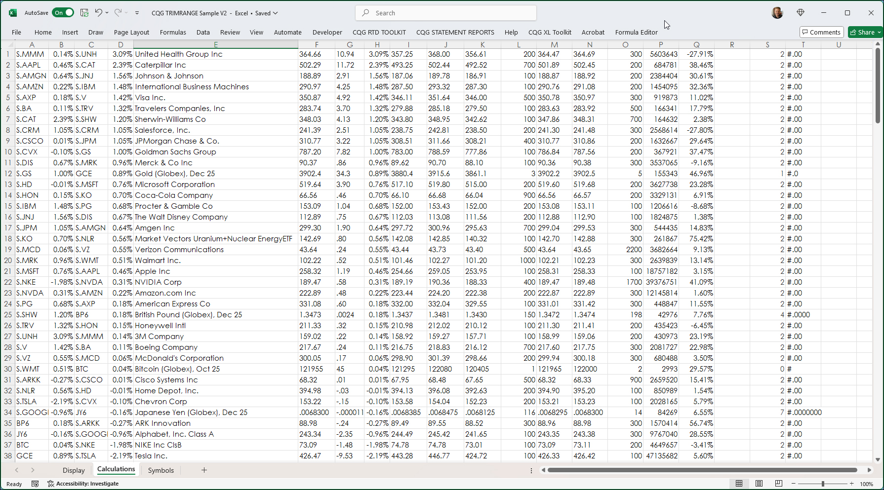
The Display tab is using the Trim Ref functions from the Calculations tab. For example, the Descriptions (Column B):
=Calculations!E.:.E
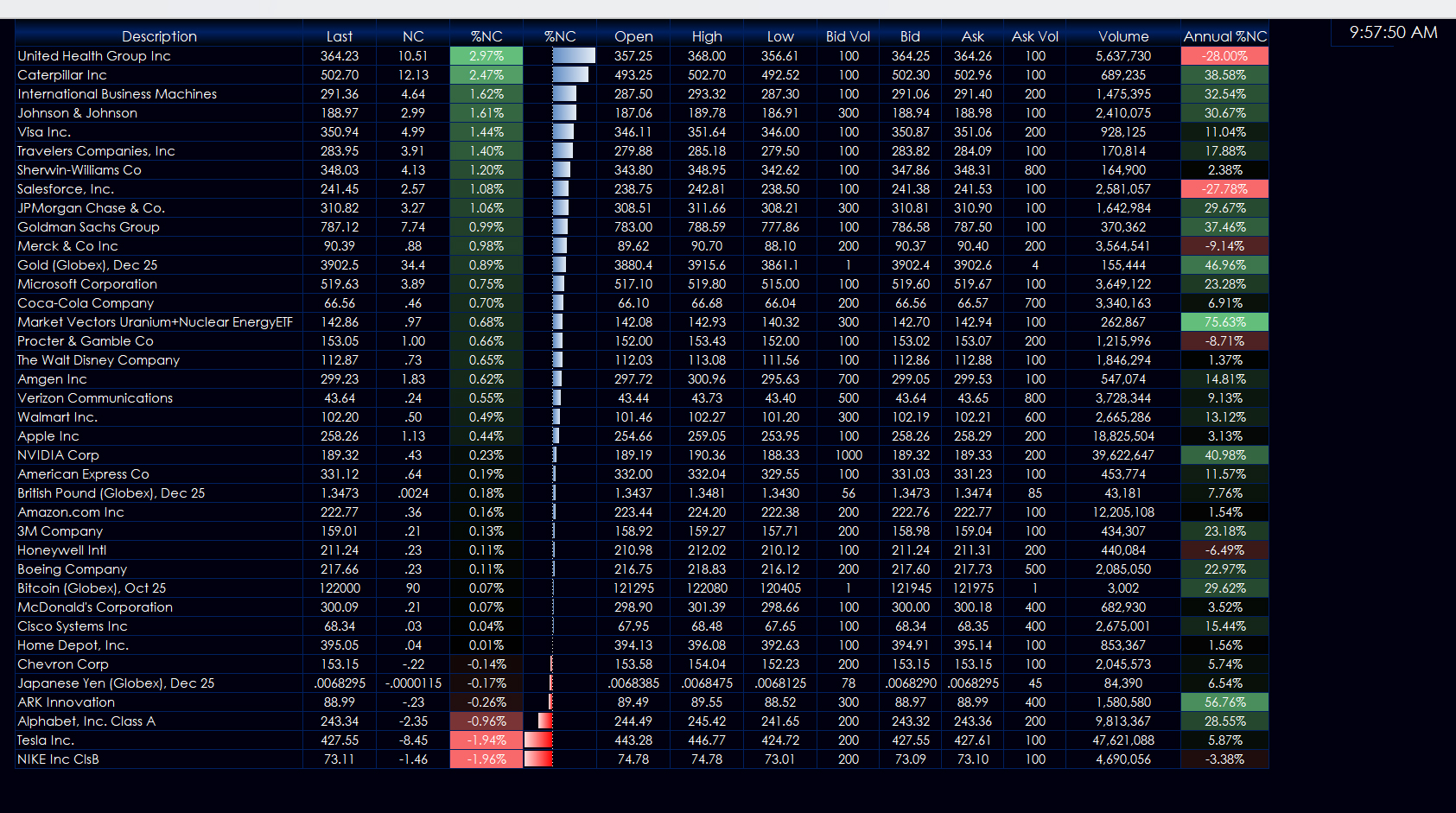
All of the columns on the Display tab are pulling in the data from the Calculations tab. The Display tab uses conditional formatting such as Heat Mapping and Data Bars.
This spreadsheet can be used as a template. Up to 200 symbols can be added on the Symbols tab. If more symbols are used, then the Calculations tab will need more RTD formula rows added to the bottom.
Requires CQG Integrated Client or CQG QTrader, data enablements for the NYSE and Nasdaq stocks. Excel 365 or more recent locally installed, not in the cloud.